
Modeling time series data can be challenging (and fascinating) due to its inherent complexity and unpredictability. Long-term trends in time series can change drastically due to certain events, for example. Recall the beginning of the global pandemic, when businesses such as airlines or brick-and-mortar shops saw a quick decline in the number of customers and sales. In contrast, e-commerce businesses continued to operate with less disruption.
Interaction terms can help model such patterns. They capture complex relationships between variables and, as a result, lead to more accurate predictions.
This post explores:
- Interaction terms in the context of time series forecasting
- Benefits of interaction terms when modeling complex relationships
- How to effectively implement interaction terms in your models
Overview of interaction terms
Interaction terms enable you to investigate whether the relationship between the target and a feature changes depending on the value of another feature. For more details, see my previous post, A Comprehensive Guide to Interaction Terms in Linear Regression.
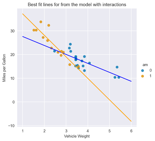
Figure 1 shows a scatterplot that represents the relationship between miles per gallon (target) and the weight of a vehicle (feature). The relationship is quite different depending on the transmission type (another feature).
Improving linear model accuracy
Without using interaction terms, a linear model would not be able to capture such a complex relationship. Effectively, it would assign the same coefficient for the weight feature, regardless of the type of transmission. Figure 1 shows the coefficients (slope of the line) by weight feature, which are drastically different for different transmission types.
To overcome this fallacy and make the linear model more flexible, add interaction terms. In general, they are a multiplication of the original features. By adding these new variables to the regression model, you can measure the effects of the interaction between them and the target.
Interaction terms in time series forecasting
Interaction terms make linear models more flexible. The following example shows how they work in the context of time series forecasting.
Prerequisites
First, load the required libraries:
import numpy as np
import pandas as pd

from sklearn.linear_model import LinearRegression

import seaborn as sns
import matplotlib.pyplot as plt
Dataset generation
Then, generate some artificial time series data with the following characteristics:
- 10 years of daily data
- Repeating patterns (seasonality) present in the time series
- A decreasing trend over the first 7 years
- No trend in the last 3 years
- Random noise, added as the last step
# for reproducibility
np.random.seed(42)
# generate the DataFrame with dates
range_of_dates = pd.date_range(
start="2010-01-01",
end="2019-12-30"
)
df = pd.DataFrame(index=range_of_dates)
# create a sequence of day numbers
df["linear_trend"] = range(len(df))
df["trend"] = 0.004 * df["linear_trend"].values[::-1]
df.loc["2017-01-01":, "trend"] = 4
# generate the components of the target
signal_1 = 10 + 4 * np.sin(df["linear_trend"] / 365 * 2 * np.pi)
noise = np.random.normal(0, 0.85, len(df))
# combine them to get the target series
df["target"] = signal_1 + noise + df["trend"]
# plot
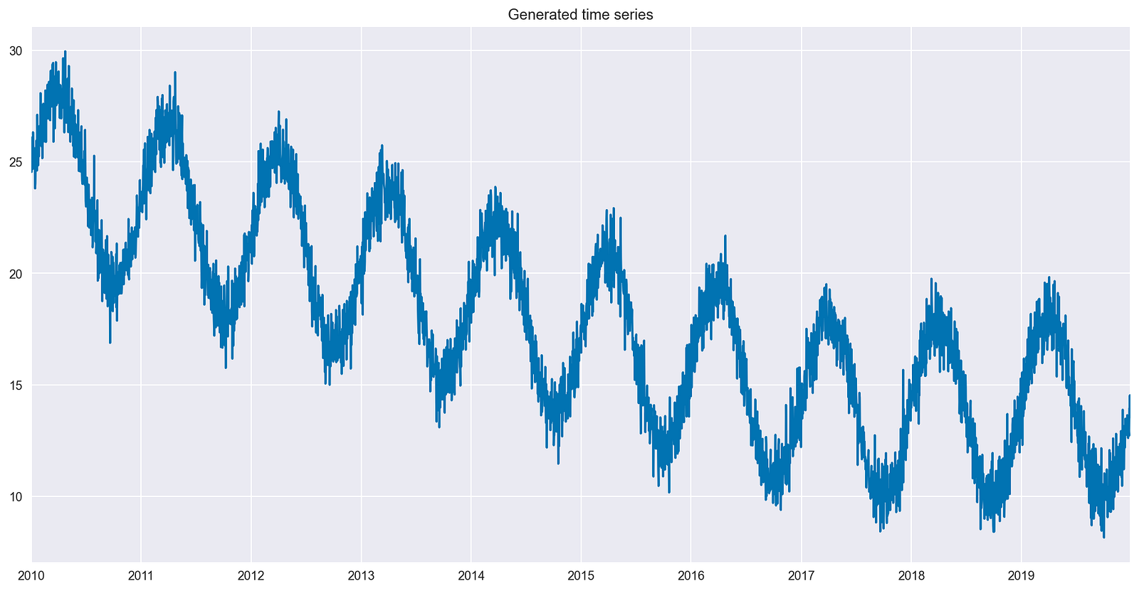
df["target"].plot(title="Generated time series");
Figure 2 shows the generated time series, which includes all the desired characteristics.
Training the benchmark model
Now train a linear model and inspect the best fit line. For this step, create very simple models with a few features. This enables you to visually inspect the impact of the interaction term on the model’s fit.
The simplest model possible contains one feature — an indicator of the passage of time. The linear_trend column created for the time series is effectively the row number of the DataFrame (ordered by date).
X = df[["linear_trend"]]
y = df[["target"]]
lm = LinearRegression()
lm.fit(X, y)
df["model_1"] = lm.predict(X)
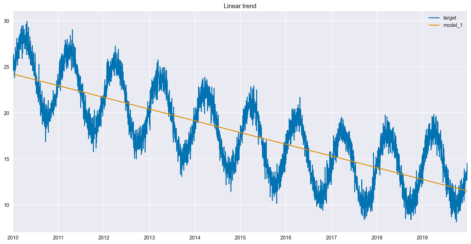
df[["target", "model_1"]].plot(title="Linear trend");
It is worth mentioning that the point is not to properly evaluate the forecasts using separate train and test sets, but rather to explain the impact of the interaction terms on the model’s fit. It is easier to observe the interaction term’s impact by inspecting the fitted values (prediction on the training set) and comparing those fitted values to the original time series.
Figure 3 shows that the linear model identified a decreasing trend for the entire time series. At the same time, the fit seems off for the last 3 years of data, as there is no trend there.
Add a breakpoint
Next, try to make the model learn the new pattern (trend change) using feature engineering. To do so, create a breakpoint, which is a placeholder variable indicating whether a given observation is after January 1, 2017. In this case, the exact point in time when the trend change happened is known.
Next, train another linear model, this time with two features:
df["after_2017_breakpoint"] = np.where(df.index >= pd.Timestamp('2017-01-01'), 1, 0)

X = df[["linear_trend", "after_2017_breakpoint"]]
y = df[["target"]]

lm = LinearRegression()
lm.fit(X, y)

df["model_2"] = lm.predict(X)

df[["target", "model_2"]].plot(title="Linear trend + breakpoint");
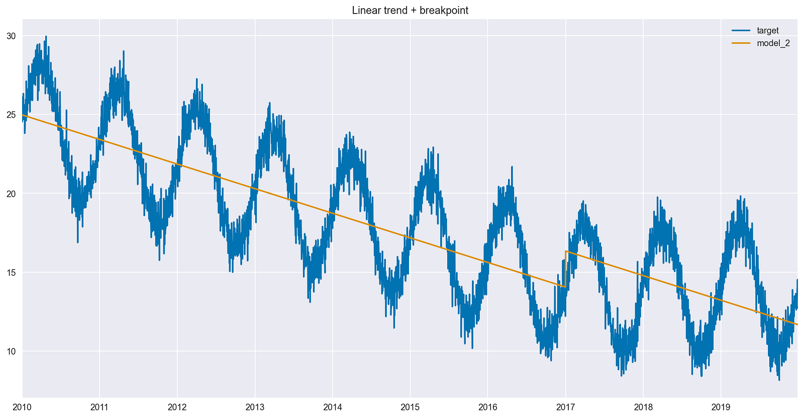
Figure 4 shows a few important changes, as listed below:
- The fitted line displays a vertical jump, which corresponds to the coefficient by the new Boolean feature.
- The vertical jump occurs exactly on the first date when the feature becomes active (a value of 1 instead of 0).
- The slope of the line is the same before and after the introduced breakpoint.
- The model is trying to compensate for the incorrect slope by adding a fixed amount to the predictions after the breakpoint.
There is no trend in the last 3 years of data, so ideally the line should be close to flat after January 1, 2017.
Adding an interaction term
To change the slope after the breakpoint, add a more complex dependency on the timestamp (represented by a linear trend). That is exactly what an interaction term does–it is a multiplication of the linear trend and the placeholder variable.
df["interaction_term"] = df["after_2017_breakpoint"] * df["linear_trend"]

X = df[["linear_trend", "after_2017_breakpoint", "interaction_term"]]
y = df[["target"]]

lm = LinearRegression()
lm.fit(X, y)

df["model_3"] = lm.predict(X)

df[["target", "model_3"]].plot(title="Linear trend + breakpoint + interaction term");
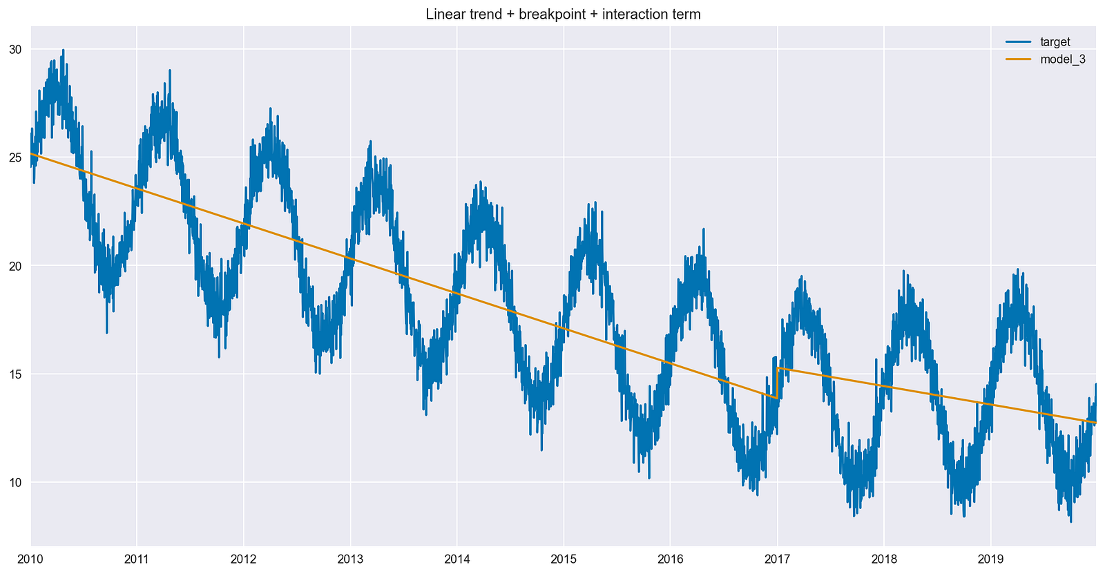
Figure 5 shows the impact of having the interaction term in the model. Compared to Figure 4, the slope of the best fit line is different after the breakpoint.
To be more precise, the difference is actually the value of the coefficient by the interaction term. While the new line did not flatten out, it is still less steep than it used to be in the earlier parts of the time series.
Introducing the breakpoint together with an interaction term increased the model’s ability to capture the trend of the time series. In turn, that should increase the predictive performance of the model.
Summary
Using interaction terms can make the specification of a linear model more flexible (different slopes for different lines), which can result in a better fit to the data and better predictive performance. You can add interaction terms as a multiplication of the original features. In the context of time series, you can use interaction terms to better capture any changes to the trend.
Find the code used in this post in A Comprehensive Guide on Interaction Terms in Time Series Forecasting on GitHub. Additionally, the code in the notebook shows how to leverage cuDF and cuML to train your models using GPU acceleration. As always, feedback is welcome. You can reach out to me on Twitter or in the comments.
