
As the fusion of AI and simulation accelerates scientific discovery, the need has arisen for a means to measure and rank the speed and throughput for building AI models of the world’s supercomputers. MLPerf HPC, now in its third iteration, has emerged as an industry-standard measure of system performance using workloads traditionally performed on supercomputers.
Peer-reviewed industry-standard benchmarks are a critical tool for evaluating HPC platforms, and NVIDIA believes access to reliable performance data will help guide HPC architects of the future in their design decisions. Developed by MLCommons, MLPerf benchmarks enable organizations to evaluate the performance of AI infrastructure across a set of important workloads traditionally performed on supercomputers.
MLPerf HPC benchmarks measure training time and throughput for three types of high-performance simulations that have adopted machine learning techniques.
This post walks through the steps the NVIDIA MLPerf team took to optimize each benchmark and measurement to extract the maximum performance. We will focus on the optimizations in MLPerf HPC v2.0 in addition to those in MLPerf HPC v1.0.
CosmoFlow
Each instance of the CosmoFlow training application benchmark loads ~8 TB of training data and ~1 TB of validation data. These consist of 512K training samples and 64K validation samples. Each sample has a 16 MB data file and a tiny 144-character label file. In total, there are over 1 million small files that need to be loaded into node-local Nonvolatile Memory Express (NVMe) before training can begin.
In MLPerf HPC v1.0, this resulted in data staging taking a significant amount of time both for strong-scale and weak-scale cases. For the weak-scale case, having many instances—each loading over 1 million files from the file system—puts additional strain on the shared disk system.
For the number of instances used for weak-scale submission, this causes a non-linear degradation of staging performance with respect to number of instances. These problems were addressed in several ways and are outlined below.
Data staging on NVMe
For a single strong training instance analysis of the NVIDIA MLPerf HPC v1.0 submission showed that only a small fraction of the maximum theoretical read bandwidth of the Selene Lustre file system was used. This was also the case for storage network interface cards (NICs) on the nodes when staging the input dataset.
During the staging phase of training, the CPU resources allocated are dedicated entirely to sourcing data from the shared file system to node-local NVMe storage. Increasing the threads dedicated to staging, and staging the training and validation data in parallel, reduced the staging time by ~75%. This equates to a ~4x speedup in staging and resulted in a 40% end-to-end reduction in total time for strong-scale.
Data compression
Loading many tiny files is inherently inefficient. In the case of CosmoFlow, there are more than 1 million files, each with 144 bytes. To further improve staging performance, the associated data and label were combined into one compressed file offline ahead of time.
In parallel with the data being staged from disk, the files are uncompressed locally onto the compute node disk. This reduces the number of files to be read from disk by 50% and the total data transferred from disk by ~85%, at the end giving an additional 13% staging speedup for strong-scale scenarios. This results in a 7% end-to-end performance improvement in overall training time for strong-scale submission.
This approach achieved over 900 GB/s read bandwidth for data staging of a strong-scale scenario.
Increasing effective bandwidth when running multiple instances
For additional algorithmic details, refer to the DeepCam explanation from the 2021 MLPerf HPC submission, MLPerf HPC v1.0: Deep Dive into Optimizations Leading to Record-Setting NVIDIA Performance.
When running multiple instances at the same time, for weak scaling, every instance must stage a copy of the training and validation data on its local nodes. This year, the NVIDIA submission implemented the distributed staging mechanism for CosmoFlow.
All of the nodes, regardless of which instance they are associated with, load a fraction of total data (1/N where N is the total number of nodes, which is 512 in this case) from the shared file system. Given the optimizations already discussed, this takes only a few seconds.
Then, every node uses MPI_Allgather to distribute the data loaded from remote storage to the other nodes that need the data. This distribution takes place over the higher bandwidth InfiniBand Fabric. In other words, a large portion of data transfer that was previously happening over the storage network is offloaded to InfiniBand Fabric with this optimization. As a result of distributing staging, staging time scales linearly with the number of instances (at least up to 128 instances) for weak-scale scenarios.
For the v1.0 submission, 32 instances were run, each staging ~9 TB of data. This took 10.76 minutes for an effective bandwidth of ~460 GB/s.
For this year’s submission, 128 instances were run, each staging ~9 TB of data, for which the total staging time takes 6.7 minutes. This means staging input data for 4x the number of instances in 1.6x less time, resulting in an effective bandwidth of ~2,900 GB/s, a 6.5x increase in effective bandwidth. Effective bandwidth assumes the amount of total data staged from the file system is the same as that of a non-distributed algorithm for a given number of instances.
Smaller instance sizes for weak-scale training
All the staging improvements enabled the size of the individual instances to be reduced for weak scaling (hence a larger number of parallel instances), which would not have been possible with the storage access bottlenecks that existed before the optimizations were implemented. In v1.0, 32 instances, each with 128 GPUs, caused the staging time to scale non-linearly. Increasing the number of instances caused a superlinear increase in staging time.
Without the improvements to efficiently stage for many instances, the staging time would have continued to grow superlinearly with the number of instances, resulting in more time being spent for data staging than the actual training.
With the optimizations described above, the number of instances were increased from 32 to 128 for the weak-scale submission, each instance using four nodes instead of 16 nodes as done in MLPerf HPC v1.0. In v2.0, staging was completed in less time, while increasing the number of models running simultaneously by 4x for weak-scale submission.
CUDA graphs and graph capture
CUDA graphs allow a single graph that consists of a sequence of kernels to be launched, instead of individually launching each of the kernels from CPU to GPU. This feature minimizes CPU involvement in each iteration, substantially improving performance by minimizing latencies—especially for strong scaling scenarios.
CUDA graphs support was recently added to PyTorch. See Accelerating PyTorch with CUDA Graphs for more details. CUDA graphs support in PyTorch resulted in around a 15% end-to-end performance gain in CosmoFlow for the strong scaling scenario, which is most sensitive to latency and jitter.
OpenCatalyst
Load balancing across GPUs
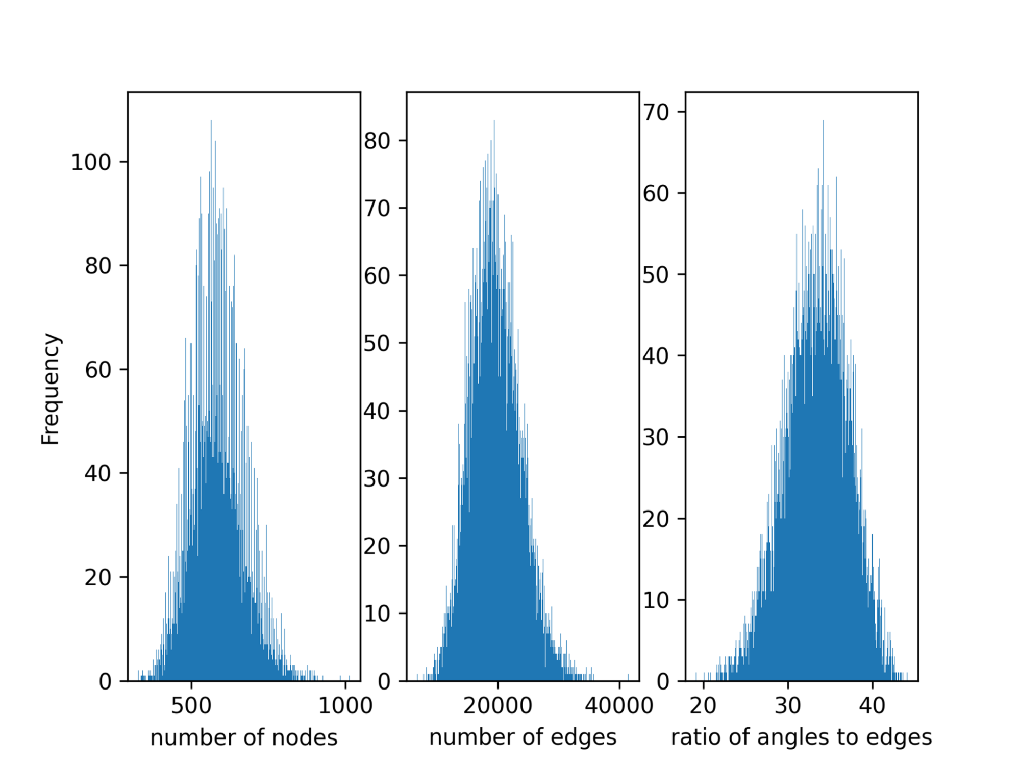
Data parallelism splits the global batch equally between each GPU. However, data-parallel task partitioning, by default, does not consider load imbalance within the batch. Load imbalance exists in Open Catalyst between the samples in a batch since the number of atoms of different molecules, the number of edges, and triplets in the graph obtained from molecules vary substantially (Figure 2).
This imbalance results in a large synchronization overhead in the multi-GPU setting. For the strong-scaling scenario, this results in 32% of the computation time being wasted. Lawrence Berkeley National Laboratory (LBNL) introduced an algorithm to balance the load across GPUs in MLPerf HPC v1.0, and this was adopted in the NVIDIA submission this round.
This algorithm first preprocesses the training data to obtain the number of edges for each sample. In the sampling stage, each GPU is given the indices of the local samples and performs a global ALLgather to get the indices of global samples.
Then the global samples are sorted by the number of edges and distributed across workers, so that each GPU processes as close to an equal number of edges as possible. This algorithm balances the workload well but introduces a large communication overhead especially as the application scales to more GPUs. This is the same algorithm used in the Open Catalyst submission from LBNL in v1.0.
NVIDIA also improved the sampling function in v2.0. The load balancing sampler avoids global (inter-GPU) communication by fetching the indices of all the samples in the global batch to all workers at the beginning. As before, samples are sorted by the number of edges, and partitioned into different buckets such that each bucket has the same approximate number of edges. Finally, each worker gets its bucket containing the indices of the samples that correspond to its global rank.
Kernel fusion using nvFuser and cuGraph-ops
There are more than 10K kernels in the original OpenCatalyst model as downloaded from MLCommons GitHub. The deep learning compiler for PyTorch, nvFuser, is a common optimization methodology that uses just-in-time (JIT) compilation to fuse multiple operations into a single kernel. The approach decreases both the number of kernels and global memory transactions.
To achieve this, NVIDIA modified the model script to enable JIT in PyTorch. Optimized fused kernels were also implemented in cuGraph-ops that were exposed through the RAPIDS framework. With the help of nvFuser and cuGraph-ops, the total number of kernels can be reduced by more than 90%.
Fusing small GEMMs to improve GPU utilization
In the original computation graph, there are many small general matrix multiplications (GEMMs) which are executed sequentially and cannot saturate the GPU. These small GEMM operations can be fused to reduce the number of kernels and improve GPU utilization. Three kinds of GEMM fusions were applied–packing, batching, and horizontal fusion–as explained below. The only change was made to the model script to implement these fusions.
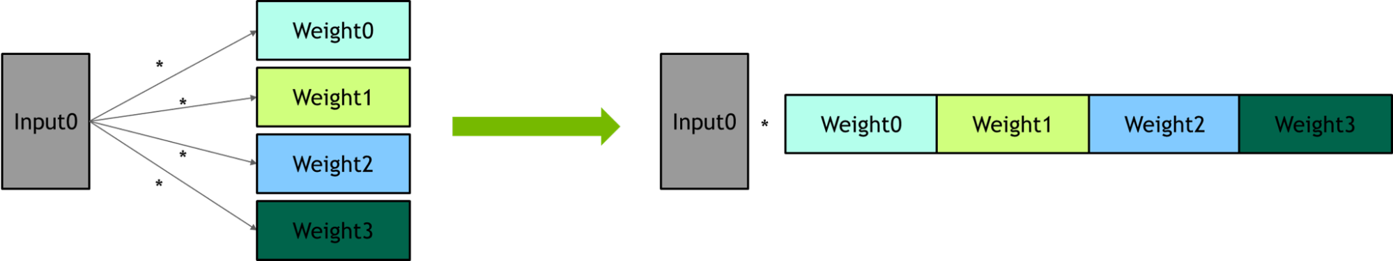
Packing – Several linear layers share the same input. One large GEMM was used to replace a set of several small GEMMs.
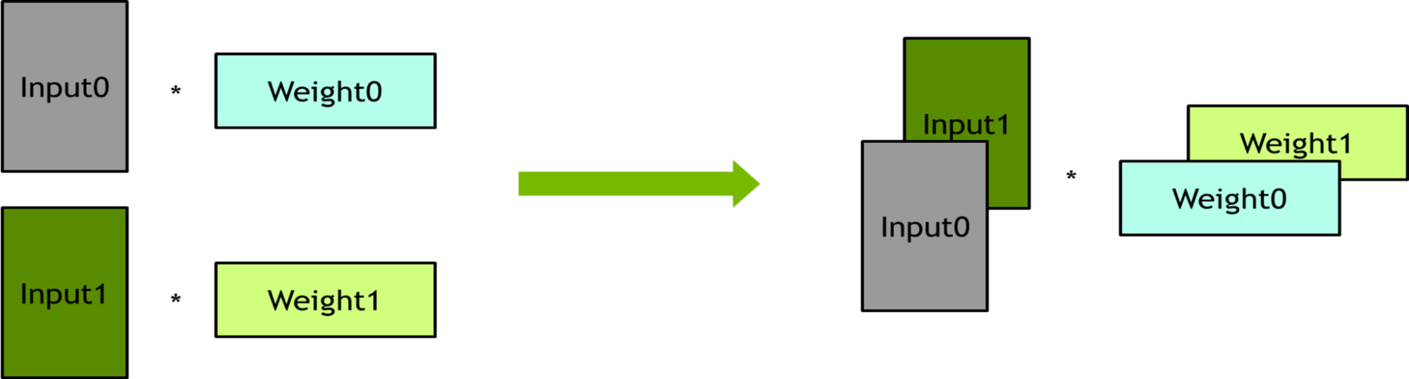
Batching – Several linear layers have no dependency on each other. These linear layers were bundled into batch operations to improve the degree of parallelism.
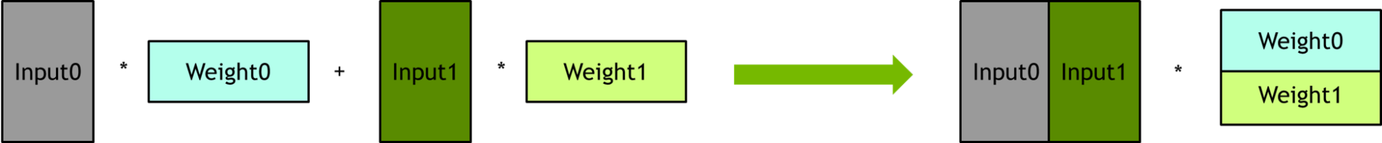
Horizontal fusion –The formula of the output reduction can be expressed as w1 x 01 + w2 x 02 + w3 x 03 + w4 x 04 + w5 x 05, which just matches the block multiplication of matrices and they can be packed together.
Eliminating redundant computation on triplets
In the original computation graph, each edge feature is expanded to triplets and then each triplet performs an elementwise multiplication. The number of triplets is about 30x the number of edges, which results in a large number of redundant computations. To remove the redundant computations, elementwise multiplication was performed on edge features first and then expanded to perform edge features to triplets.
Pipeline optimization
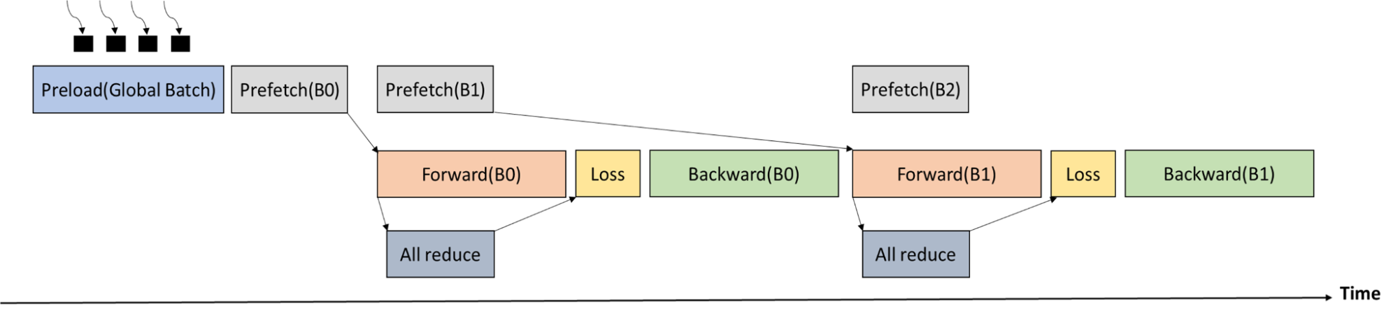
An ALLReduce communication across all the workers is required before the loss stage to obtain the total number of atoms in the current global batch. As the execution time of forward pass is longer than the execution time of ALLReduce, the communication can be well overlapped.
Figure 6 shows the training process timeline. The global batch is first loaded by multiple processes into CPU memory. Memcpy from CPU memory to GPU memory and ALLReduce (to get the number of atoms in the global batch) are overlapped with forward pass.
Data staging
The training data of the Open Catalyst benchmark is 300 GB, and one DGXA100 node has a system memory of 2,048 GB and 256 threads (128 threads per socket, with two sockets per node). As a result, the whole training data can be preloaded into the CPU memory at the beginning. There is no need to load the minibatch from disk to CPU memory in every training step.
To accelerate data preload, NVIDIA launched 256 processes, each loading 300/256 (~1.2) GB of the training dataset. It took about 10s~15s to finish the preload, which is negligible with respect to the end-to-end training time.
DeepCam
Loading data
Previously, the transparent in-memory data loader utilized background processes to cache data locally in dynamic random-access memory (DRAM). This causes a large overhead, and thus the loader was reimplemented to employ threads instead.
Performance was previously limited by the Python Global Interpreter Lock (GIL). This time, the C++ based IO helper class was optimized to release the GIL. This approach allows the background loading to overlap with other CPU work. The same optimization was applied to the distributed data stager for the weak scaling score, improving end-to-end performance by about 15%.
Full iteration CUDA graph capture
Compared to MLPerf HPC v1.0, the scope of CUDA graph capture was extended to the full iteration, forward and backward pass, optimizer, and learning rate scheduler step. For this purpose, the sync-free optimizer FusedMixedPrecisionLAMB and DistributedLAMB from the NVIDIA APEX packages were employed for weak and strong scaling benchmarks.
Additionally, all DeepCAM learning rate schedulers were ported to GPU. By increasing the fraction of the computation that is executed inside the CUDA graph, performance variability across devices that stems from CPU execution variability is reduced. Scale-out performance improves as a result.
Distributed optimizer
For improving strong scaling performance, the DistributedLAMB optimizer was used. This optimizer is especially suited for small per-GPU local batch sizes and large scales, since optimizer cost is more pronounced in such settings. The performance gain at scale is about 3% end-to-end for DeepCAM.
cuDNN kernel optimizations
DeepCAM features a large number of computing kernels with different performance characteristics. While NVIDIA improved the performance of grouped convolutions in v1.0, the performance of pointwise convolutions was also improved in v2.0. They are used together with the grouped convolutions to form depth-wise separable convolutions.
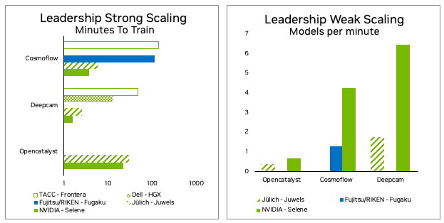
MLPerf HPC v2.0 final results
AI is changing how science is done with high performance computing. Each year, new and more accurate surrogate models are built and shown to vastly outpace physics-based simulations with sufficient accuracy to be useful. Protein folding and the advent of OpenFold, RoseTTAFold, and AlphaFold 2 have been revolutionized by this AI-based approach, bringing protein structure-based drug discovery within reach.
MLPerf HPC reflects the supercomputing industry’s need for an objective, peer-reviewed method to measure and compare AI training performance for use cases relevant to HPC.
NVIDIA has made significant progress since the MLPerf HPC v1.0 submission in 2021. The Selene supercomputer shows that the NVIDIA A100 Tensor Core GPU and the NVIDIA DGX-A100 SuperPOD, though nearly three years old, are still the best system for AI training for HPC use cases and beyond.
For more information, see MLPerf HPC Benchmarks Show the Power of HPC+AI.
