
NVIDIA cuOpt is an accelerated optimization engine for solving complex routing problems. It efficiently solves problems with different aspects such as breaks, wait times, multiple cost and time matrices for vehicles, multiple objectives, order-vehicle matching, vehicle start and end locations, vehicle start and end times, and many more.
More specifically, cuOpt solves multiple variants of two problems: the Capacitated Vehicle Routing Problem with Time Windows (CVRPTW) and the Pickup and Delivery Problem with Time Windows (PDPTW). The objective of these problems is to serve customer requests while minimizing the number of vehicles and total distance traveled in respective order.
cuOpt has broken 23 world records set in the past three years on the largest routing benchmarks, as verified by SINTEF.
This post explores key elements of optimization algorithms and their definitions and the process of benchmarking NVIDIA cuOpt against leading solutions in the field, highlighting the significance of these comparisons. Throughout the post, we use the term ‘request’ for an order for CVRPTW and for a pickup-delivery order pair for PDPTW problems.
Although there are various constraints and problem dimensions in this domain, the scope of this post is limited to capacity and time windows constraints. Capacity constraints enforce that the total commodities present at the vehicle at any time cannot exceed the vehicle capacity. Time window constraints enforce that the orders are serviced at a time not earlier than the beginning of the time window and not later than the end of the time window.
Combinatorial optimization
Combinatorial optimization problems are among the most computationally expensive problems in the world (NP-hard), with the number of possible states in the search space being factorial. As it is not possible to use exact algorithms for large problems, heuristics are used that approximate the solution toward the optimal point. Heuristics explore the search space using various algorithms that are computationally expensive with quadratic or higher computational complexity.
High complexity and the nature of the problem enable the acceleration of these algorithms using massively parallel GPUs. Thanks to GPU acceleration, it is possible to obtain close-to-optimal solutions in a reasonable time.
Building evolutionary route optimization algorithms
A typical routing solver consists of two phases: generating the initial solution and improving the solution. This section describes the procedures to generate initial solutions and to improve them.
Initial solution generation algorithm
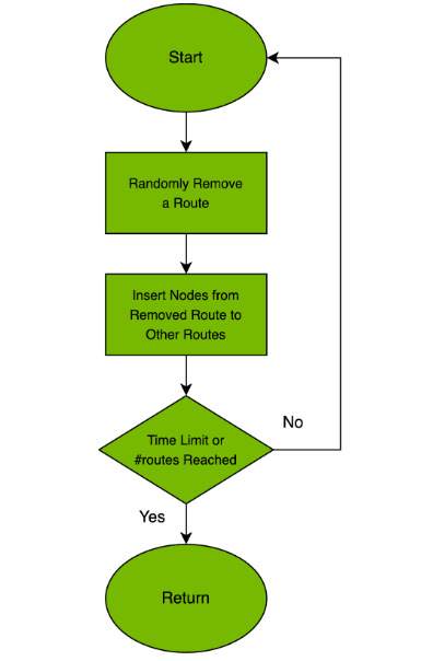
Generating a feasible initial solution with a limited fleet that meets all the constraints is an NP-hard problem itself. Our team has improved and parallelized the Guided Ejection Search (GES) algorithm to place the requests to routes.
The main idea of the GES is simple. We first try to insert a request to the route. If it’s not feasible to insert that request, we eject one or more easy-to-insert requests from a route and insert the request to the relaxed route. A penalty score (p-score) for each request indicates the difficulty of inserting that request into a route. The algorithm inserts a request only if the sum of the p-scores of ejected requests is smaller than the considered request.
Each time it’s not possible to insert a request into a route, even with ejections, we increment the p-score of that request and try again. We keep all the unserved requests in an ejection pool and the algorithm runs until the ejection pool is empty. In other words, it runs until all requests are served.
The main drawbacks of this algorithm are cycling (returning to the previous set of nodes in the solution), slow rate of finding ejection combinations when the number of ejected nodes is high, and considering only weak, randomly perturbed solutions. We have removed those setbacks, which has enabled us to generate solutions with a much lower number of routes than the current state-of-the-art methods.
Before we dive deeper into the ejection algorithms, it is crucial to understand that feasibility checks and solution evaluations are performed at constant time using the time warp method. Although this approach significantly reduces the computation time, it also makes the parallelization more difficult because of the need to obey the lexicographic order of the search of an arbitrary number of ejections.
Finding which requests to eject and where to insert the considered request feasibly is a computationally expensive problem: it is exponential with respect to the number of ejected requests and requires checking all the insertion positions in all routes. Our experiments show that a small number of ejections causes the cycling of the algorithm.
Thus, we propose a method that enables ejecting as many as 10 requests (heuristically) and five requests when an extensive search is performed—in parallel. We parallelize the ejection algorithm by ejecting a fragment from each route and handling these temporary routes in a thread block. Then, we try to insert the considered request to all possible positions in parallel.
The deep search algorithm tries all possible permutations of ejections of all requests in a route. We use different thread blocks for each request insertion position and perform the lexicographic search in parallel by splitting the lexicographical order into independent sub-permutations.
The GES algorithm loops until we exhaust the time limit or the pool of requests is empty. At every iteration, we perturbate the solution to improve the solution state and to open gaps in the solution so that a feasible insertion can be found. The perturbation is a random local search that randomly relocates and swaps nodes between and within the route.
After the optimal number of vehicles is found to fulfill the requests, we switch to the improvement phase, which is responsible for minimizing the objective. By default, this is the total traveled distance, but it is possible to configure other objectives in cuOpt.
Evolutionary process and local search algorithms
The improvement phase works on multiple solutions and improves them using evolutionary strategies. Generated solutions are placed in a population. To reach initial solutions that are diverse enough, we use randomization in the generation process. Utilizing the GPU architecture, we generate many diverse solutions in parallel. The diverse population runs through an evolutionary improvement process, with the best properties of the solutions kept in the newer generations.
In a single step of the evolutionary process, we take two random solutions and apply a crossover operator. This generates an offspring solution that inherits good properties from both parents. Different crossover operators can be applied to the solutions, some of which leave the offspring in an incomplete state. We repair the solution by ejecting duplicate nodes, inserting unrouted nodes or fixing the infeasibility by doing an infeasibility local search on it.
For example, the order-based crossover operator reorders the nodes in one or multiple routes of one parent solution with respect to the order they appear in another parent solution. The resulting offspring conserves the grouping properties of one parent and ordering properties of another solution. The result of this particular operator is a complete solution that is probably infeasible with respect to time and capacity constraints. cuOpt contains multiple crossover operators that are executed randomly on solutions.
The local search phase after the crossovers plays a crucial role in reducing or eliminating the infeasibility or improving the total objective, or distance traveled, in this case. The objective weights of the local search are determined by what is important to optimize. Higher weights on infeasibility help return solutions to the feasible region, which is usually the case for most problems.
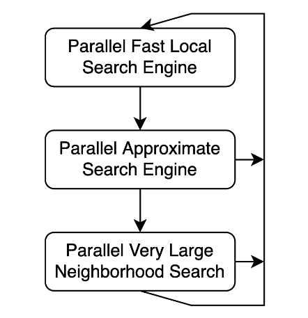
Local search finds a local minimum for the offspring solution, which then participates in further evolutionary steps. It is crucial to have a fast local search, as it is the main factor in how many improvement iterations can be done within the time budget. We use fast, approximate, and large neighborhood search algorithms to find a good local minimum while being performant. Instead of performing a fixed-size neighborhood local search as in classical approaches, we have designed a “net” that catches easy improvements quickly, and very deep operators when stagnation is reached.
Fast operators quickly explore small neighborhoods, while approximate operators can evaluate different moves each time they are applied. This is particularly important because the crossovers frequently leave some routes intact. A large neighborhood operator moves requests in a chain of moves expressed as a move cycle among routes, as explained in A GPU Parallel Algorithm for Finding a Negative Subset Disjoint Cycle in a Graph.
The cyclic operators explore a very large neighborhood where it is not possible to explore with simple operators. This is simply because the constraints prohibit these simple operators from passing some of the hills in the search space. This workflow enables the use of fast operators often and more computationally expensive deep operators less frequently.
GPU parallelization is done by mapping each of the hypothetical routes to a thread block. This enables the use of shared memory to store route-related data, which is temporary while searching for the moves. The temporary route is either a copy of the original route or a version where one or more requests are ejected. Threads in the thread block try to insert all possible requests from other routes to all positions in the temporary route.
After finding and recording all the moves, we find the best move per route pair by summing up the insertion/ejection cost delta of each. The cost delta is calculated by the objective weights, which contain infeasibility penalization weights as well. We execute multiple such moves if they are exclusive of each other in terms of the routes they modify.
Benchmarking cuOpt
We have continuously improved the performance and the quality of cuOpt. To measure the quality, we have benchmarked the solver against the best-known solutions on the most studied benchmarks, including Gehring & Homberger for CVRPTW and Li & Lim for PDPTW. In practice, how quick the solver can reach the desired solutions is important for companies.
Evaluation criteria and goal
- Accuracy is defined as the percent gap between the found solution and the best known solutions (BKS) in terms of objectives. The problem specification states the first objective as the vehicle count and the second objective as the traveled distance.
- The time to solution measure states how much time is needed to reach a certain gap to BKS or desired objective result. Time to solution is one of the most important criteria for practical use cases. It is important to reach a high-accuracy solution within the time budget. The combinatorial optimization algorithms take a significant amount of time.
Figures 3 and 4 show the convergence behavior of the solver on a subset of large instances of benchmarks.
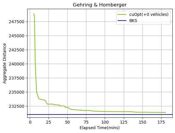
We have selected one instance from each of the categories (C1_10_1, C2_10_1, R1_10_1, R2_10_1, RC1_10_1, RC2_10_1) to show the overall behavior of the solver depending on the (clustered, random) and (long route, short route) instances. The aggregate sum that is sampled every minute is compared to aggregate BKS.
The steep convergence at the beginning yields to slowly approaching the aggregate BKS as time passes. For these sets of instances, we were able to match the aggregate vehicle count of the BKS. The cuOpt solver can find the BKS vehicle counts in almost all instances of Gehring & Homberger instances. However, the actual performance depends on the time spent at the initial solution generation compared to the improvement phase.
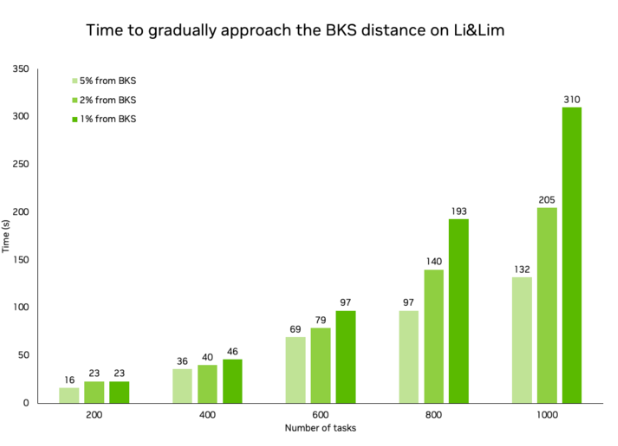
While the solver converges quickly on larger instances, it converges orders of magnitude faster on smaller instances. In the following tables, we show how much time it takes to reach the BKS for various problem sizes while achieving the same vehicle count as BKS for all of them.
cuOpt sets 23 world records
With the new approach of GPU-accelerated heuristics and cutting-edge evolutionary strategies, cuOpt has broken the records for 15 instances from the Gehring & Homberger benchmark and eight instances from the Li & Lim benchmark.
NVIDIA now holds all the records for CVRPTW and PDPTW categories for the past three years.
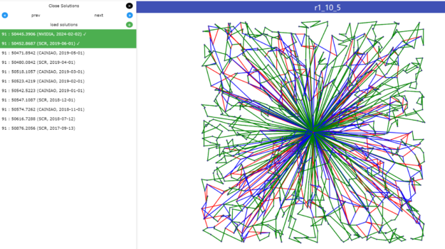
In Figure 5, each edge represents the path from one task to another. Green lines represent edges common to the previous record. Blue and red edges are different between two solutions. Thanks to evolutionary strategies, the cuOpt solutions are in a completely different place in the search space of possible solutions, meaning that there are many different edges.
The overall average gap to BKS for Gehring & Homberger is -0.07% distance gap and 0.29% vehicle count gap. The overall average gap to BKS for Li & Lim is 1.22% distance gap and 0.36% vehicle count gap. The benchmarks were run for 200 minutes on a single NVIDIA H100 GPU.
Conclusion
NVIDIA cuOpt achieves high-quality solutions in seconds with GPU acceleration and NVIDIA technologies like RAPIDS. We have achieved speedups of 100x in the local search operations, compared to a CPU-based implementation. CPU-based solvers require hours to reach similar solutions.
Learn more and get started with NVIDIA cuOpt. You can also explore the model through the NVIDIA API catalog and NVIDIA LaunchPad. And discover how cuOpt can help your organization save time and money.
Join us for the NVIDIA GTC 2024 session, Advances in Optimization AI to hear from NVIDIA Optimization AI Engineering Manager Alex Fender. You can also take the NVIDIA Deep Learning Institute Training, Learn How to Use Our Route Optimization Microservice to Drive Efficiency and Cost Savings.
