MLPerf is an industry-wide AI consortium tasked with developing a suite of performance benchmarks that cover a range of leading AI workloads widely in use. The latest MLPerf v1.0 training round includes vision, language and recommender systems, and reinforcement learning tasks. It is continually evolving to reflect the state-of-the-art AI applications.
NVIDIA submitted MLPerf v1.0 training results for all eight benchmarks, as is our tradition. In fact, systems built upon the NVIDIA AI platform are the only commercially available systems to make submissions across the board.
Compared to our previous MLPerf v0.7 submissions, we improved up to 2.1x on a chip-to-chip basis and up to 3.5x at scale. We set 16 performance records with eight on a per-chip basis and eight at-scale training in the commercially available solutions category.
| Benchmark | Max Scale Records (min) DGX SuperPod | Per Accelerator Records (min) A100 |
| Recommendation (DLRM) | 0.99 | 15.3 |
| NLP (BERT) | 0.32 | 169.2 |
| Image classification (ResNet-50 v1.5) | 0.4 | 219.0 |
| Speech recognition – Recurrent (RNN-T) | 2.75 | 309.6 |
| Image Segmentation (3D U-Net) | 3.00 | 229.1 |
| Object detection lightweight (SSD) | 0.48 | 66.5 |
| Object detection heavyweight (Mask R-CNN) | 3.95 | 400.2 |
| Reinforcement Learning | 15.53 | 2156.3 |
(*) Per Accelerator performance for A100 computed using NVIDIA 8xA100 server time-to-train and multiplying it by 8 | Per Chip Performance comparisons to others arrived at by comparing performance at the closest similar scale.
Per-Accelerator Records: BERT: 1.0-1033 | DLRM: 1.0-1037 | Mask R-CNN: 1.0-1057 | ResNet50 v1.5: 1.0-1038 | SSD: 1.0-1038 | RNN-T: 1.0-1060 | 3D U-Net: 1.0-1053 | MiniGo: 1.0-1061
Max Scale Records: BERT: 1.0-1077 | DLRM: 1.0-1067 | Mask R-CNN: 1.0-1070 | ResNet50 v1.5: 1.0-1076 | SSD: 1.0-1072 | RNN-T: 1.0-1074 | 3D U-Net: 1.0-1071 | MiniGo: 1.0-1075
MLPerf name and logo are trademarks. For more information, see www.mlperf.org.
This is the second MLPerf training round featuring NVIDIA A100 GPUs. Our continual year-over-year improvement on the same hardware is a lively testament to the strength of the NVIDIA platform and commitment to continuous software improvement. As in previous MLPerf rounds, NVIDIA engineers developed a host of innovations to achieve these new levels of performance:
- Extending CUDA Graphs across all benchmarks. Neural networks are traditionally launched as individual kernels from the CPU to execute on the GPU. In MLPerf v1.0, we launched the entire sequence of kernels as a graph on the GPU, minimizing communication with the CPU.
- Using SHARP to double the effective interconnect bandwidth between nodes. SHARP offloads collective operations from the CPU and GPU to the network and eliminates the need for sending data multiple times between endpoints.
The CUDA graph and SHARP enhancements enabled us to increase our scale to a record number of 4096 GPUs used to solve a single AI network.
- Spatial parallelism enabled us to split a single image across eight GPUs for massive image segmentation networks like 3D U-Net and to use more GPUs for higher throughput.
- Among hardware improvements, new HBM2e GPU memory on the NVIDIA A100 GPU increased memory bandwidth by nearly 30% to 2 TBps.
This post provides insights into many of the optimizations used to deliver the outstanding scale and performance. Many of these improvements are available on NGC, which is the hub for NVIDIA GPU-optimized software. You can realize the benefits of these optimizations in your real-world applications, instead of just observing better benchmark scores from the sideline.
At-scale training
Large-scale training requires system hardware and software to be precisely tuned to work together and support the unique performance requirements that arise at scale. NVIDIA made major advances on both dimensions, which are now available for production use.
On the system side, the key building block of our at-scale training is the NVIDIA DGX SuperPOD. DGX SuperPOD is the culmination of years of expertise in HPC and AI data centers. It is based on the NVIDIA DGX A100 with the latest NVIDIA A100 Tensor Core GPU, third-generation NVIDIA NVLink, NVSwitch, and the NVIDIA ConnectX-6 VPI 200 Gbps HDR InfiniBand. These were combined to make Selene a top 5 supercomputer in the Top 500 supercomputer list, with the following components:
- 4480 NVIDIA A100 Tensor Core GPUs
- 560 NVIDIA DGX A100 systems
- 850 Mellanox 200G HDR InfiniBand switches
On the software side, the NGC container release v. 21.05 enhances and enables several capabilities:
- Distributed optimizer support enhancement.
- Improved communication efficiency with Mellanox HDR Infiniband and NCCL 2.9.9.
- Added SHARP support. SHARP improves upon the performance of MPI and machine learning collective operations. SHARP support was added to NCCL to offload all-reduce collective operations into the network fabric, reducing the amount of data traversing between nodes.
Workloads
In this section, we dive into the optimizations for selected individual MLPerf workloads.
Recommendation (DLRM)
Recommendation is arguably the most pervasive AI workload in data centers today. The NVIDIA MLPerf DLRM submission was based on HugeCTR, a GPU-accelerated recommendation framework that is part of the NVIDIA Merlin open beta framework. The HugeCTR v3.1 beta release added the following optimizations:
- Hybrid embedding
- Optimized collectives
- Optimized data reader
- Overlapping MLP with embedding
- Whole-iteration CUDA graph
Hybrid embedding
One of the major challenges in scaling DLRM to multiple nodes is the ~10x difference in per-GPU all-to-all bandwidth between NVLink and Infiniband. This makes the embedding exchange between nodes a significant bottleneck during training.
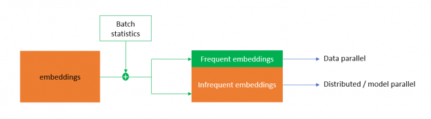
To counteract this, HugeCTR implemented hybrid embedding, a novel embedding design that deduplicates the categories in a batch before doing the embedding weight exchange in the forward pass. It also reduces the gradients locally before doing gradient exchange in the backward pass.
For efficient deduplication, the hybrid embedding maps the categories to frequent and infrequent embeddings based on the statistical access frequency of categories. The frequent embedding is implemented in a data-parallel fashion that takes away most of the replicated categories in a batch, reducing the embedding exchange traffic. Infrequent embedding follows the distributed model parallel-embedding paradigm. This enables DLRM to scale to multiple nodes with unprecedented efficiency.
Optimized collectives
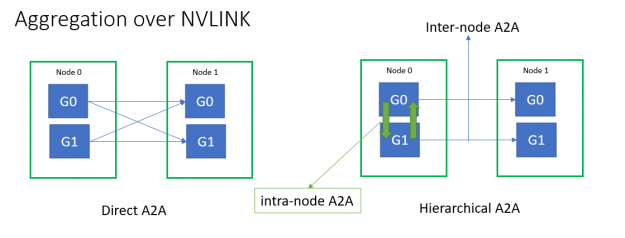
All-to-all and all-reduce collective latencies play a significant role in scaling efficiency. Multinode all-to-all throughput for small message sizes was limited by the Infiniband message rate. To mitigate this, HugeCTR implemented fused NVLink aggregation using hierarchical all-to-all for embedding exchange.
You can optimize internode all-to-all and all-reduce latencies further:
- Directly using the native IB verbs API and SHARP to mitigate library overheads.
- Graph-capturable, GPU-initiated communication to reduce launch overheads.
- One-sided eager protocol instead of two-sided rendezvous protocol to reduce network hops.
- Eliminating redundant message buffer copies using persistent communication buffers.
- Reduced NIC-GPU synchronization latency using NIC atomics directly on GPU memory instead of indirection through CPU.
Intranode all-reduce is also optimized using a single-shot reduction algorithm as opposed to ring.
Frequent embedding all-reduce and MLP all-reduce are fused into a single all-reduce operation to save on exposed all-reduce latency.
Optimized data reader
Input pipeline plays a significant role in training performance. To achieve peak I/O throughput, HugeCTR implemented a fully asynchronous data reader using the Linux asynchronous I/O library (AIO). Because hybrid embedding requires the whole batch to be present on all the GPUs, direct host-to-device (H2D) for each GPU would make PCIe a bottleneck. So, the data is copied onto the GPUs using a hierarchical approach, by first doing a H2D over PCIe and then a broadcast over NVLink.
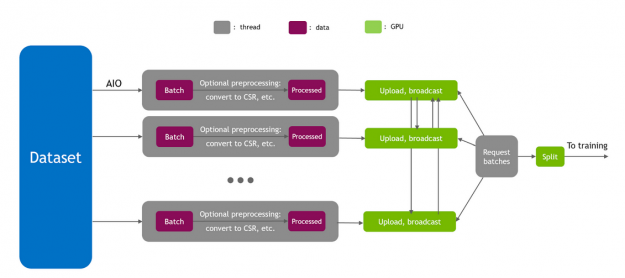
Moreover, H2D traffic from data readers may interfere with internode all-to-all and all-reduce traffic over PCIe. So, HugeCTR implements intelligent data-reader scheduling to avoid such interference.
Overlapping MLP with embedding
Because the bottom MLP has no data dependencies with embedding, several components of the bottom MLP could be overlapped with embedding for efficient utilization of GPU resources.
- Bottom MLP forward is overlapped with the embedding forward pass
- Frequent embedding local weight update is overlapped with all-reduce
- MLP weight update is overlapped with internode all-to-all
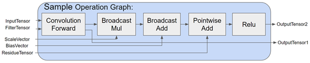
cuBLASLt GEMM fusions
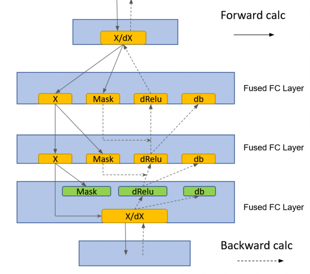
HugeCTR implemented a fused, fully connected layer that made use of cublasLt GEMM fusions:
- GEMM + Relu + bias fusion for MLP fprop
- GEMM + dRelu + dBias fusion for MLP bprop
Whole-iteration CUDA graph
To reduce launch latencies and prevent PCIe interference between kernel launches, data-reader, and communication traffic, all DLRM compute and communication kernels are designed to be stream-capturable. The whole training iteration is captured into a single CUDA graph.
With the preceding optimizations, we scaled to multiple nodes and completed the DLRM training task in just under a minute on 14 DGX-A100 nodes. This is a 3.3x speedup compared to the previous v0.7 submission.
NLP (BERT)
BERT is arguably one of the most important workloads in the NLP domain today. In the MLPerf v1.0 round, we improved upon our v0.7 submission with the following optimizations:
- Fused multihead attention
- Distributed LAMB
- Synchronization-free training
- CUDA Graphs in PyTorch
- One-shot all-reduce with SHARP
Fused multihead attention
The size of the activation tensors inside the multihead attention block grows with the square of the sequence length. This results in increased memory footprint, as well as longer runtimes due to the accompanying memory access operations. We fused softmax, masking, and dropout operations into a single kernel both in forward pass and backward pass. By doing so, we avoided several memory access operations for large activation tensors inside the multihead attention block, which resulted in a meaningful performance boost.
For more information, see SelfMultiheadAttn in the NVIDIA Apex library.
Distributed LAMB
In this MLPerf round, we implemented distributed LAMB. In distributed LAMB, the gradients are first split across eight GPUs within each DGX-A100 node. This is followed by an all-reduce between the nodes in eight separate groups. After this operation, each GPU has one of eight chunks that constitute the all-reduced gradient tensor, and the LAMB optimizer is run on 1/8th of the full gradient tensor.
When necessary, gradient norms are computed by computing local norms and performing an all-reduce operation. After the optimizer, an intranode all-gather operation is performed at each node, so that each GPU has the full updated parameter tensor. Execution is continued with the forward pass of the next iteration.
Distributed LAMB substantially improves performance both for single-node and multinode configurations. For more information, see DistributedFusedLAMB in the Apex library.
Synchronization-free training
There are cases where the GPU execution depends on some value that is stored or calculated on the CPU. An example is when a specific tensor has a varying size that depends on the computation for each iteration. Because tensor size information is kept on the CPU, there must be a synchronization between GPU and CPU to pass the tensor size information for proper buffer allocation.
Our solution was using a tensor with fixed size, but indicating which elements are valid using a separate Boolean mask. With this approach, no CPU-GPU synchronization was needed, as the tensor sizes are known. When a subsequent computation must know the real size of the tensor, as for an averaging operation, the elements of the Boolean mask can be summed on the GPU.
Even though this approach resulted in slightly more access to GPU memory, it is much faster than having CPU synchronization in the critical path. This optimization resulted in a significant performance boost for small local batch size, which is the case for our max-scale configuration. This is because CPU synchronizations can’t keep up with fast GPU execution for small batch sizes.
Another source of CPU-GPU synchronization is the data that is kept on CPU, such as learning rate or potentially other optimizer states. We kept all the optimizer states on the GPU for distributed LAMB to achieve synchronization-free execution.
As a result of these optimizations, we eliminated all the synchronizations between CPU and GPU during a training cycle. The only synchronizations are the ones that happen at the evaluation points, to log the evaluation accuracy in a file in real time for every evaluation point.
CUDA Graphs in PyTorch
Traditionally, CPU launches each GPU kernel individually. In general, even though GPU kernels do more work for large batch sizes, CPU kernel launch work and related CPU overheads stay fixed, barring the variations in CPU scheduling. As a result, for small local batch sizes, CPU overhead can become a significant performance bottleneck. This is what happened in our max-scale BERT configuration in MLPerf.
On top of that, when CPU execution becomes a bottleneck, variations in CPU execution result in different runtimes across all GPUs for each iteration. This introduces a significant synchronization overhead when the workload is scaled to many GPUs (4096 GPUs in this case). Each GPU synchronizes every iteration for gradient reductions, and iteration time is determined by the slowest worker.
CUDA Graphs is a feature that enables launching an entire sequence of kernels at one time, eliminating CPU overheads between kernel executions. CUDA Graphs recently became available in PyTorch. By graph capturing the model, we eliminated CPU overhead and the accompanying synchronization overhead. The CUDA Graphs implementation resulted in a 1.7x performance boost just by itself for our max-scale BERT configuration.
One-shot all-reduce with SHARP
SHARP improved the performance of collectives significantly for BERT, especially for our max-scale configuration. End-to-end performance boost from SHARP is 17% for this BERT configuration.
Image classification (ResNet-50 v1.5)
ResNet-50 is the veteran among MLPerf workloads. In this edition of MLPerf, we continue to optimize ResNet by improving Conv+BN+ReLu fusion kernels in CuDNN, along with the following optimizations:
DALI optimizations
At large scales (>128 nodes) for ResNet-50, we reduced the local batch size per GPU to extremely small values. This often results in sub-20-ms iteration time. To reduce the overhead of the data pipeline, we introduced the input batch multiplier (IBM). DALI throughput is higher at large batch sizes than smaller batch sizes. To take advantage of this fact, we created super batches that are much larger than the local batch size. For each iteration, we then derived the needed samples from these super batches, increasing the DALI processing throughput and reducing the data pipeline overhead.
At these small iteration times, gapless and continuous execution is the key to perfect scaling. Pre-allocating DALI buffers through hints is another feature that we introduced to reduce the overhead of dynamic GPU memory allocation while exploring the dataset.
MXNet fused BN+ReLu and BN+Add+ReLu performance optimizations
For ResNet-50, batch norm (BN) is a significant portion of the network’s iteration time. We optimized the fused BN+ReLu and BN+Add+ReLu kernels in MXNet through vectorization, cache-friendly memory traversals, and reducing quantization.
Improved MXNet dependency engine improvements
The new MXNet dependency engine provides an asynchronous approach to scheduling work on the GPU, reducing the host (CPU) overhead and jitter such as overhead arising from MXNet and Horovord handshake.
In the new dependency engine, the operation updates the dependency as soon as the work is scheduled on the GPU, not when the work is finished. It is the subsequent operation that must perform the synchronization to ensure correctness. This is further enhanced by removing the need for synchronization and using cudaStreamWait events to manage dependencies.
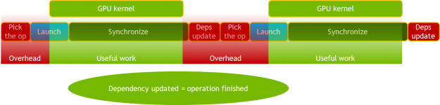
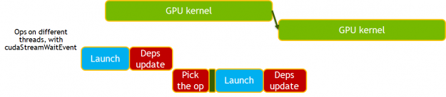
Image segmentation (3D U-Net)
U-Net3D is one of the two new workloads in this round of MLPerf training. We used the following optimizations:
Spatial parallelism
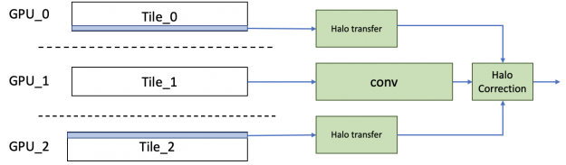
In 3D U-Net, because the sample number in the training dataset is relatively small, there is a fundamental limit to how much it can be scaled with naive data parallelism. To break that limit, we used spatial parallelism to split a single image across eight GPUs. At the end of the backward propagation, the gradients from each partition can be all-reduced as usual to get the resultant gradients, which can then be used to calculate the weight gradients.
The naive approach to implementing spatial parallel convolution is to transfer the halo information from the neighboring GPU before running the convolution. However, to increase efficiency, we implemented a different scheme, in which we transfer the halo from the neighboring GPU in parallel to running the main inner convolutions. The error term to this main convolution is calculated independently using the halo and added to get the result. By hiding the transfer costs, we saw much better scaling efficiency than with the naive approach.
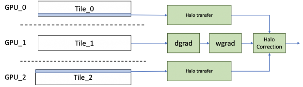
For the backward propagation, similarly, the halos needed for the dgrad operation are transferred in parallel with the computation of the weight gradients and data gradients. The halos transferred for the data gradients are then reused for computing the correction terms for both weight and data gradients.
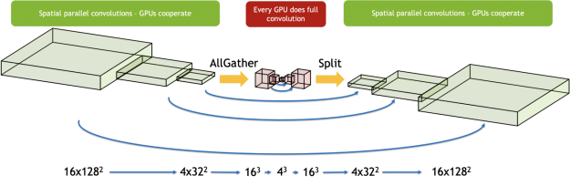
3D U-Net has a bottleneck region in the middle of the network with much smaller activation sizes, which are not suited for spatial parallelism. We used a hybrid approach where we used spatial parallelism only for the layers that benefit from it. We gathered the activations for the sample from all GPUs right before this bottleneck region and executed these layers serially on each GPU. We split the work among the GPUs again when cooperating became beneficial. This made sure that we made the best choice separately for each region of the network.
Asynchronous evaluation
Evaluation contributes a significant amount of time in the reference code. Because evaluation can be run concurrently with training, we assigned dedicated nodes for running just evaluation.
To hide the evaluation behind the training cycle entirely, we used spatial parallelism to speed up the validation step. In addition, as evaluation uses the same set of images, the images were loaded only one time and then cached in the GPU memory.
Because the evaluation doesn’t start until a third of the way through the training, the evaluation nodes have enough time to load, process, and cache the dataset, as well as initialize all required libraries.
At the end of the training cycle, training nodes use InfiniBand to transfer the model quickly to the evaluation nodes and continue running subsequent training iterations. The evaluation nodes run evaluation after the model parameters are transferred. At the end of the evaluation, the evaluation node communicates to the training nodes if the target accuracy is reached.
The number of evaluation nodes added are just enough to hide the entire evaluation cycle behind the training cycle.
![Asynchronous evaluation runs concurrently with training on dedicated nodes.]](https://developer-blogs.nvidia.com/wp-content/uploads/2021/06/Asynchronous-evaluation-schedule-625x217.png)
Data loader
We optimized the data loader in two ways: optimizing the augmentations and caching the dataset.
Augmentations: 3D U-Net requires heavy augmentation due to the small size of the dataset. One of the most expensive operations is something that we call “biased crop”. On contrary to a random crop, biased crop selects regions with a positive label with a given probability. This requires heavy computations of 3D-connected components on labels every time the expensive path is selected. To avoid calculating the connected components every time that the sample is loaded, the result is cached in the host and reused so that it is calculated only one time.
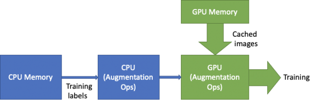
Data loading: As the training gets faster with the new features, the I/O starts to show up as the bottleneck. To alleviate this, we cached the entire image dataset in the GPU memory. This removes the PCIe and I/O from the critical data loader path. While the images are loaded from the large and high-bandwidth GPU memory, the labels are loaded from the CPU to perform augmentations.
Channels-Last layout support
Because the Channels-Last layout is more efficient for convolution kernels, native support for the Channels-Last format was added in MXNet. This avoids any additional transposes needed in the model to take advantage of highly efficient GPU kernels.
Optimized CuDNN kernels
3D U-Net has multiple encoder and decoder layers with small channel counts. Using a typical tile size of 256×64 for the kernels used in these operations results in significant tile-size quantization effects. To optimize this, cuDNN added kernels optimized for smaller tile sizes with better cache reuse. This helped 3D U-Net achieve better compute utilization.
Apart from these optimizations, 3D U-Net benefited from the optimized BatchNorm + ReLu activation kernel. The BatchNorm kernel was run repeatedly with a BatchSize value of 1 to get the Instance-Norm functionality. The asynchronous dependency engine implemented in MXNet, CUDA Graphs, and SHARP also helped performance significantly.
With the array of optimizations made for 3D U-Net, we scaled to 100 DGX A100 nodes (800 GPUs), with training running on 80 nodes (640 GPUs) and evaluation running on 20 nodes (160 GPUs). The max-scale configuration of 100 nodes got over 9.7x speedup as compared to the single-node configuration.
Object detection (lightweight) (SSD)
This is the fourth time that the lightweight SSD has been featured in MLPerf. In this round, the evaluation schedule was changed to happen every fifth epoch, starting from the first. In previous rounds, the evaluation scheduled started from the 40th epoch. Even with the extra computational requirement, we sped up our submissions time by more than x1.6.
SSD consists of many smaller convolution layers. The benchmark was particularly affected by the improvements to the MXNet dependency engine, CUDA Graphs, and the enablement of SHARP, as discussed earlier.
More efficient configs
The training time of a deep learning model is a multivariable function. In its most basic form, the equation is as follows:
\(Train\; Time = Average\; Iteration\; Time\; \cdot\; Number\; of\; Iterations\)
The goal is to minimize \(Train\; Time\) where both it and \(Average\; Iteration\; Time\) and \(Number\; of\; Iterations\) are functions of the batch size.
\(Average\; Iteration\) is a monotonically non-decreasing function. Batch sizes are more computationally efficient, but they take more time per iteration.
On the other hand, \(Number\; of\; Iterations\), up to a certain batch size, is a monotonically nonincreasing function. Larger batch sizes require fewer iterations to converge because the model sees more images per iteration.
| Batch size | Iterations per epoch (1) | Epochs to convergence (2) | Total iterations |
| 1024 | 115 | 50 | 5750 |
| 2048 | 58 | 65 | 3770 |
| 3072 | 39 | 75 | 2925 |
| 4096 | 29 | 90 | 2610 |
(1) MS-COCO epoch size is 117266 images; (2) empirical value
Compared to the v0.7 submission where we used a batch size of 2048, the v1.0 batch size was 3072, which required 22% fewer iterations. Because the larger iteration was only 20% slower, the result was an 8% faster time to convergence.
In this example, going to a batch size of 4096 instead of 3072 would’ve resulted in a longer training time. The 11% fewer iterations didn’t make up for the extra 20% run time per iteration.
Optimized evaluation
Evaluation can be broken into two phases:
- Inference: Using the trained model to make predictions against the validation dataset. Runs on the GPU.
- Scoring: Evaluating the inference results against the ground truth. Runs asynchronously on the CPU.
The new evaluation in v1.0 adds eight validation cycles to the base submission. Worse, improvements to the epoch train time means that scoring needs to take less than 2 seconds or the training time of five epochs. Otherwise, it won’t be fully hidden and any training time improvements are pointless.
To improve inference time, we made sure that the inference graph was static. We improved the nonmaximum suppression implementation and moved the Boolean mask, used to filter negative detections, to outside the graph. Static graphs save memory reallocation time and make switching between training and inference contexts faster.
For scoring, we used nv-cocoapi, which is a C++ implementation of cocoapi and 60x times faster. For v1.0, we improved the nv-cocoapi performance by 2x with multithreaded results accumulation, faster indices sorting, and caching the ground truth data structures.
Object detection (heavyweight) (Mask R-CNN)
We optimized object detection with the following techniques:
- CUDA Graphs in PyTorch
- Removing synchronization points
- Asynchronous evaluation
- Dataloader optimization
- Better fusion of ResNet layers with CUDNN v8
CUDA Graphs in PyTorch
Deep learning frameworks use GPUs to accelerate computations, but a significant amount of code still runs on CPU cores. CPU codes process metadata like tensor shapes to prepare arguments needed to launch GPU kernels. Processing metadata is a fixed cost while the cost of the computational work done by the GPUs is positively correlated with batch size. For large batch sizes, CPU overhead is a negligible percentage of total run time cost. At small batch sizes, CPU overhead can become larger than GPU run time. When that happens, GPUs go idle between kernel calls.
This issue can be identified on an Nsight Systems timeline plot. The plot below shows the “backbone” portion of Mask R-CNN with per-GPU batch size of 1 before graphing. The green portion shows CPU load while the blue portion shows GPU load. In this profile, you see that the CPU is maxed out at 100% load while GPU is idle most of the time. There is a lot of empty space between GPU kernels.
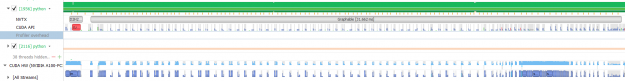
CUDA graph is a tool that can automatically eliminate CPU overhead when tensor shapes are static. A complete graph of all kernel calls is captured during the first step. In subsequent steps, the entire graph is launched with a single operation, eliminating all the CPU overhead. PyTorch now has support for CUDA graph, we used this to speed up Mask R-CNN for MLPerf 1.0.
![With CUDA graph, the entire graph is launched with a single op, eliminating all the CPU overhead.]](https://developer-blogs.nvidia.com/wp-content/uploads/2021/06/CUDA-graph-optimization.png)
With graphing, we see that the GPU kernels are tightly packed and GPU utilization remains high. The graphed portion now runs in 6 ms instead of 31 ms, a speedup of 5x. We mostly just graphed the ResNet backbone, not the entire model. Even then, we saw >2x uplift for the entire benchmark just from graphing.
Removing synchronization points
There are many PyTorch modules that make the main process wait until the GPU has finished all previously launched kernels. This can be detrimental to performance, because it makes the CPU sit idle when it could be working on launching more kernels. The CPU can get ahead of the GPU in low overhead segments and start launching kernels from succeeding segments. As long as total CPU overhead is less than total GPU kernel time, the CPU never becomes the bottleneck, but this breaks when sync points are introduced. Also, model segments that have sync points cannot be graphed with CUDA graph, so removing syncs is important.
We did some of this work for MLPerf 1.0. For instance, torch.randperm was rewritten to use CUB instead of Thrust because the latter is a synchronous C++ template library. These improvements are available in the latest NGC container.
Removing all the syncs improved the uplift that we saw from CUDA Graphs from 1.6x to 2.5x.
Asynchronous evaluation
Our MLPerf 0.7 submission did asynchronous evaluation, but it wasn’t fast enough to keep up with training after optimizations. Evaluation took 18 seconds per epoch, and 4 seconds of that was fully exposed time. Without changes to the evaluation code, our at-scale submission would have clocked in about 100 seconds slower.
Of the three evaluation phases, inference and prep account for all the exposed time. To speed up inference, we cached the test images in GPU memory, as they never change. We moved the prep phase to a pool of background processes, as each sample in the test dataset can be processed independently. We scored segmentation masks and boxes simultaneously in two background processes. These optimizations reduced evaluation time to ~4 seconds per epoch.
Dataloader optimization
This component loads and augments images during training. In our MLPerf 0.7 submission, all data loading work was done by CPU cores. The old dataloader was not fast enough to keep up with training after optimizations. To remedy that, we developed a hybrid dataloader.
The hybrid dataloader decodes the images on CPU and then does image augmentation work on GPU using Torchvision. To hide the cost of dataloading completely, we moved the load next image call in the main training loop after the loss backward call. The CPUs are idle for several milliseconds after the loss backward call because of theCUDA Graph launch. This is more than enough time to decode the next image. After the GPUs finish back propagation, they sit idle while the optimizer does all-reduce on the gradients. During this idle time, the dataloader does image augmentation work.
Better fusion of ResNet layers with CUDNN v8
The basic building block of ResNet50 is a three layer-stack composed of a convolution, batch norm, and activation function. For Mask R-CNN, the batch norm is frozen, which means that both the batch norm and activation function are pointwise operations that can be fused.
In previous rounds, we used the PyTorch JIT fuser to fuse the two pointwise operations. Thanks to the new fusion engine in CUDNN v8, we improved on this by fusing the pointwise operations with the convolution. The flexible API of the fusion engine also enabled us to fuse all three basic layers under one autograd function. That let us work around a limitation of the fuser by doing asymmetric fusions in backpropagation for an even bigger performance boost.
Speech recognition (RNN-T)
Speech recognition with RNN-T is the other new workload in this round of MLPerf training. We used the following optimizations:
- Apex transducer loss
- Apex transducer joint
- Sequence splitting
- Batch splitting
- Batch evaluation with CUDA Graphs
- More optimized LSTMs in cuDNN v8
Apex transducer loss
RNN-T uses a special loss function that we call transducer loss function. The algorithm that computes the loss is iterative in nature. A naive implementation is often inefficient due to the irregular memory access pattern and the exposed long memory read latency.
To overcome this difficulty, we developed apex.contrib.transducer.TransducerLoss. It uses a diagonal-wave-front-like computing paradigm to exploit the parallelism in the algorithm. Shared memory and registers are used extensively to cache the data exchanged between iterations. The loss function also employs prefetch to hide the memory access latency.
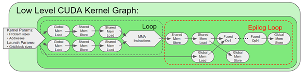
Apex transducer joint
Another component that is often found in a transducer-type network is the transducer joint operation. To accelerate this operation, we developed apex.contrib.transducer.TransducerJoint. This Apex extension is not only faster than its native PyTorch counterpart, but also enables output packing, reducing the workload seen by following layers.
Figure 17 shows the packing operation by the Apex transducer joint. In the baseline joint operation, the paddings from the input sequences are carried over to the output, as the joint operation is oblivious to the input padding. In the Apex transducer joint operation, the paddings are removed at the output, reducing the size of the tensor fed to the following operations.
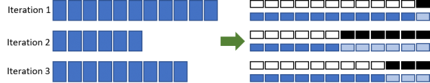
Sequence splitting
To reduce computations of LSTMs that are wasted on paddings, we split batch processing into two phases (Figure 18). In the first pass, all the samples in the minibatch up to certain time steps (enclosed by the black boxes) are evaluated. Half of the samples in the minibatch are completed in the first pass. The remaining time steps of the other half of the samples (enclosed by the red boxes) are evaluated in the second pass. The regions enclosed by blue boxes represent the savings from batch splitting.
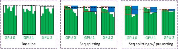
The black dashed line in Figure 18 estimates the workload seen by the GPUs. Because the batch size is halved for the second pass, the workload seen by the GPU is roughly halved. In multi-GPU training, it is often the slowest GPU that limits the training throughput. The dashed line is obtained from the GPU with most workloads.
To mitigate this load imbalance, we employed a technique called presorting, where samples in a minibatch are sorted based on their sequence lengths. The longest and shortest sequences are placed on the same GPU to balance the workload. The intuition behind this is that GPUs with long sequences are likely to be the bottleneck. Therefore, short sequences should be placed on these GPUs as well to maximize the benefit of sequence splitting.
Batch splitting
RNN-T has an interesting network structure where the LSTMs deal with relatively small tensors, whereas the joint net takes much larger tensors. To enable LSTMs to run more efficiently with a large batch size while not exceeding the GPU memory capacity by having a huge tensor in the joint net, we employed a technique called batch splitting (Figure 17). We used a reasonably large batch size so that LSTMs achieved a decent GPU utilization. In contrast, joint net operates on a portion of the batch and loops through those subbatches one by one.
In Figure 19, a batch splitting factor of 2 is used. In this case, the batch sizes of the inputs to the LSTMs and the joint net are B and B/2, respectively. Because all the tensors generated by the joint net, except the gradients for the weights, are no longer needed after the backpropagation is completed, they can be released and create room for the next subbatch in the loop.
![Batch splitting enables LSTMs to run more efficiently with a large batch size while not exceeding the GPU memory.]](https://developer-blogs.nvidia.com/wp-content/uploads/2021/06/Batch-splitting-625x286.png)
Batch evaluation with CUDA Graphs
Other than accelerating training, evaluation of RNN-T has also been scrutinized. The evaluation of RNN-T is iterative in nature and the evaluation of the predict network is performed step by step. Each sample in a batch might pick different code paths in the same time step, depending on the execution results. Because of these, a naive implementation leads to a low GPU utilization rate and a long evaluation time that is comparable to the training itself.
To overcome these difficulties, we performed two categories of optimizations in the evaluation. The first optimization performed evaluation in batch mode and take care of the different control flows in a batch with predicates. The second optimization graphed the main RNN-T evaluation loop, which consists of many short GPU kernels. We also used loop unrolling and overlapping CPU-GPU communication with GPU execution to amortize associated overheads. The optimized evaluation was more than 100x faster than the reference code for the single-node configuration, and more than 30x faster for the max-scale configuration.
More optimized LSTMs in cuDNN v8
LSTM is the main building block of RNN-T. A large portion of the end-to-end network time is spent on LSTMs. In cuDNN v8, the performance of LSTMs has been heavily optimized. For example, better horizontal fusion algorithms and heuristics were applied to the GEMMs in LSTM cells and drop out in between LSTM layers, improving performance and reducing the overhead from dropout.
Summary
MLPerf v1.0 showcases the continuous innovation happening in the AI domain. The NVIDIA AI platform delivers leadership performance with tight integration of hardware, data center technologies, and software to realize the full potential of AI.
In the last two-and-a-half years since the first MLPerf training benchmark launched, NVIDIA performance has increased by nearly 7x. The NVIDIA platform excels in both performance and usability, offering a single leadership platform from data center to edge to cloud.
All software used for NVIDIA submissions is available from the MLPerf repository, to enable you to reproduce our benchmark results. We constantly add these cutting-edge MLPerf improvements into our deep learning frameworks containers available on NGC, our software hub for GPU-optimized applications.
