
 The performance of GPU architectures continue to increase with every new generation. Modern GPUs are so fast that, in many cases of interest, the time taken by each GPU operation (e.g. kernel or memory copy) is now measured in microseconds. However, there are overheads associated with the submission of each operation to the GPU – also at the microsecond scale – which are now becoming significant in an increasing number of cases.
Real applications perform large numbers of GPU operations: a typical pattern involves many iterations (or timesteps), with multiple operations within each step. For example, simulations of molecular systems iterate over many timesteps, where the position of each molecule is updated at each step based on the forces exerted on it by the other molecules. For a simulation technique to accurately model nature, typically multiple algorithmic stages corresponding to multiple GPU operations are required per timestep. If each of these operations is launched to the GPU separately, and completes quickly, then overheads can combine to form a significant overall degradation to performance.
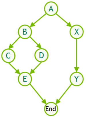
CUDA Graphs have been designed to allow work to be defined as graphs rather than single operations. They address the above issue by providing a mechanism to launch multiple GPU operations through a single CPU operation, and hence reduce overheads. In this article, we demonstrate how to get started using CUDA Graphs, by showing how to augment a very simple example.
The Example
Consider a case where we have a sequence of short GPU kernels within each timestep:
Loop over timesteps
    …
    shortKernel1
    shortKernel2
    …
    shortKernelN
    …
We are going to create a simple code which mimics this pattern. We will then use this to demonstrate the overheads involved with the standard launch mechanism and show how to introduce a CUDA Graph comprising the multiple kernels, which can be launched from the application in a single operation.
First, let’s write a compute kernel as follows:
#define N 500000 // tuned such that kernel takes a few microseconds

__global__ void shortKernel(float * out_d, float * in_d){
  int idx=blockIdx.x*blockDim.x+threadIdx.x;
  if(idx<N) out_d[idx]=1.23*in_d[idx];
}
This simply reads an input array of floating point numbers from memory, multiplies each element by a constant factor, and writes the output array back to memory. The time taken by this kernel depends on the array size, which has been set to 500,000 elements such that the kernel takes a few microseconds. We can use the profiler to measure the time taken to be 2.9μs, where we are running on an NVIDIA Tesla V100 GPU using CUDA 10.1 (and we have set the number of threads per block as 512 threads). We will keep this kernel fixed for the remainder of the article, varying the way in which it is called.
First Implementation with Multiple Launches
We can use the above kernel to mimic each of the short kernels within a simulation timestep as follows:
#define NSTEP 1000
#define NKERNEL 20

// start CPU wallclock timer
for(int istep=0; istep<NSTEP; istep++){
  for(int ikrnl=0; ikrnl<NKERNEL; ikrnl++){
    shortKernel<<<blocks, threads, 0, stream>>>(out_d, in_d);
    cudaStreamSynchronize(stream);
  }
}
//end CPU wallclock time
The above code snippet calls the kernel 20 times, each of 1,000 iterations. We can use a CPU-based wallclock timer to measure the time taken for this whole operation, and divide by NSTEP*NKERNEL which gives 9.6μs per kernel (including overheads): much higher that the kernel execution time of 2.9μs.
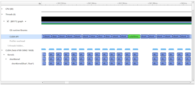
Note the existence of the cudaStreamSynchronize call after each kernel launch, which means that each subsequent kernel is not launched until the previous completes. This means that any overheads associated with each launch will be fully exposed: the total time will be the sum of the kernel execution times plus any overheads. We can see this visually using the Nsight Systems profiler:

This shows a section of the timeline (with time increasing from left to right) including 8 consecutive kernel launches. Ideally, the GPU should remain busy with minimal idle time, but that is not the case here. Each kernel execution is seen towards the bottom of the image in the “CUDA (Tesla V100-SXM2-16G)” section. It can be seen that there are large gaps between each kernel execution, where the GPU is idle.
We can get more insight by looking at the “CUDA API” row which shows GPU-related activities from the CPU’s perspective. The purple entries in this row correspond to time that the CPU thread spends in the CUDA API function which launches the kernel, and the green entries are time spent in the CUDA API function which synchronizes with the GPU, i.e. waiting for the kernel to be fully launched and completed on the GPU. So, the gaps between the kernels can be attributed to a combination of CPU and GPU launch overheads.
Note that, on this timescale (where we are inspecting very short events), the profiler adds some additional launch overhead, so for accurate analysis of performance, a CPU-based wallclock timer should be used (as we do throughout this article). Nevertheless, the profiler is effective in providing an insightful overview of the behavior of our code.
Overlapping Kernel Launch and Execution
We can make a simple but very effective improvement on the above code, by moving the synchronization out of the innermost loop, such that it only occurs after every timestep instead of after every kernel launch:
// start wallclock timer
for(int istep=0; istep<NSTEP; istep++){
  for(int ikrnl=0; ikrnl<NKERNEL; ikrnl++){
    shortKernel<<<blocks, threads, 0, stream>>>(out_d, in_d);
  }
  cudaStreamSynchronize(stream);
}
//end wallclock timer
The kernels will still execute in order (since they are in the same stream), but this change allows a kernel to be launched before the previous kernel completes, allowing launch overhead to be hidden behind kernel execution. When we do this, we measure the time taken per kernel (including overheads) to be 3.8μs (vs 2.9μs kernel execution time). This is substantially improved, but there still exists overhead associated with multiple launches.
The profiler now shows:
It can be seen that we have removed the green synchronization API calls, except the one at the end of the timestep. Within each timestep it can be seen that launch overheads are now able to overlap with kernel execution, and the gaps between consecutive kernels have reduced. But we are still performing a separate launch operation for each kernel, where each is oblivious to the presence of the others.
CUDA Graph Implementation
We can further improve performance by using a CUDA Graph to launch all the kernels within each iteration in a single operation.
We introduce a graph as follows:
bool graphCreated=false;
cudaGraph_t graph;
cudaGraphExec_t instance;
for(int istep=0; istep<NSTEP; istep++){
  if(!graphCreated){
    cudaStreamBeginCapture(stream, cudaStreamCaptureModeGlobal);
    for(int ikrnl=0; ikrnl<NKERNEL; ikrnl++){
      shortKernel<<<blocks, threads, 0, stream>>>(out_d, in_d);
    }
    cudaStreamEndCapture(stream, &graph);
    cudaGraphInstantiate(&instance, graph, NULL, NULL, 0);
    graphCreated=true;
  }
  cudaGraphLaunch(instance, stream);
  cudaStreamSynchronize(stream);
}
The newly inserted code enables execution through use of a CUDA Graph. We have introduced two new objects: the graph of type cudaGraph_t contains the information defining the structure and content of the graph; and the instance of type cudaGraphExec_t is an “executable graph”: a representation of the graph in a form that can be launched and executed in a similar way to a single kernel.
So, first we must define the graph, and we do this by capturing information on GPU activities that are submitted to the stream between the cudaStreamBeginCapture and cudaStreamEndCapture calls. Then, we must instantiate the graph through the cudaGraphInstantiate call, which creates and pre-initialises all the kernel work descriptors so that they can be launched repeatedly as rapidly as possible. The resulting instance can then be submitted for execution through the cudaGraphLaunch call.
Crucially, it is only necessary to capture and instantiate once (on the first timestep), with re-use of the same instance on all subsequent timesteps (as controlled here by the conditional statement on the graphCreated boolean value).
Therefore, we now have the following procedure:
- First step:
- create and instantiate graph
- launch graph (comprising 20 kernels)
- wait for graph to complete
- For each of the remaining 999 steps
- launch graph (comprising 20 kernels)
- wait for graph to complete
Measuring the time taken for this complete process, and dividing by 1000×20 to give an effective time per kernel (including overheads), gives 3.4μs (vs 2.9μs kernel execution time), so we have successfully further reduced the overheads. Note that in this case, the time to create and instantiate the graph is relatively large at around 400μs, but this is only performed a single time, so this is only contributes around 0.02μs to our per-kernel cost. Similarly, the first graph launch is around 33% slower that all subsequent launches, but that becomes insignificant when re-using the same graph many times. The severity of the initialization overhead is obviously problem dependent: typically in order to benefit from graphs you need to re-use the same graph enough times. Many real-world problems involve substantial repetition, and are therefore suitable for use of graphs.
The remaining overheads are due to the necessary steps required to launch each graph on the GPU, and we expect to further reduce these with future improvements to CUDA. We intentionally don’t show any profile here since we are still working on CUDA Graph compatibility with the profiling tools. With the current CUDA release, the profile would look similar to that shown in the “Overlapping Kernel Launch and Execution” except there would only be one “cudaGraphLaunch” entry in the CUDA API row for each set of 20 kernel executions, and there would be extra entries in the CUDA API row at the very start corresponding to the graph creation and instantiation. Each of these 20 kernels would still be shown as individual entries, but in order to provide such a picture, the profiler currently disables some graph-related optimizations. A more accurate profile would not disable any optimizations and represent each set of 20 kernels through display of a single graph entry.
Further Information
It is nice to observe benefits of CUDA Graphs even in the above very simple demonstrative case (where most of the overhead was already being hidden through overlapping kernel launch and execution), but of course more complex cases provide more opportunities for savings. Graphs support multiple interacting streams including not just kernel executions but also memory copies and functions executing on the host CPUs, as demonstrated in more depth in the simpleCUDAGraphs example in the CUDA samples.
The example in this article used the stream capture mechanism to define the graph, but it is also possible to define the nodes and dependencies explicitly through newly available API calls – the simpleCUDAGraphs sample shows how to implement the same problem using both techniques. Furthermore, graphs may also span multiple GPUs.
Implementation of multiple activities within a single graph, as opposed to treating each activity separately, ultimately provides more information to CUDA and hence more opportunities for optimization. For more information, please refer to the CUDA Graphs section of the Programming Guide and watch the GTC 2019 talk recording CUDA: New Features and Beyond.