Energy Efficiency in High-Performance Computing: Balancing Speed and Sustainability

The world of computing is on the precipice of a seismic shift.

The demand for computing power, particularly in high-performance computing (HPC), is growing year over year, which in turn means so too is energy consumption. However, the underlying issue is, of course, that energy is a resource with limitations. So, the world is faced with the question of how we can best shift our computational focus from performance to energy efficiency.

When considering this question, it is important to take into account the correlation between task completion rate and energy consumption. This relationship is often overlooked, but it can be an essential factor.

This post explores the relationship between speed and energy efficiency, and the implications should the shift to completing tasks more quickly ‌occur.

Take transportation for example.

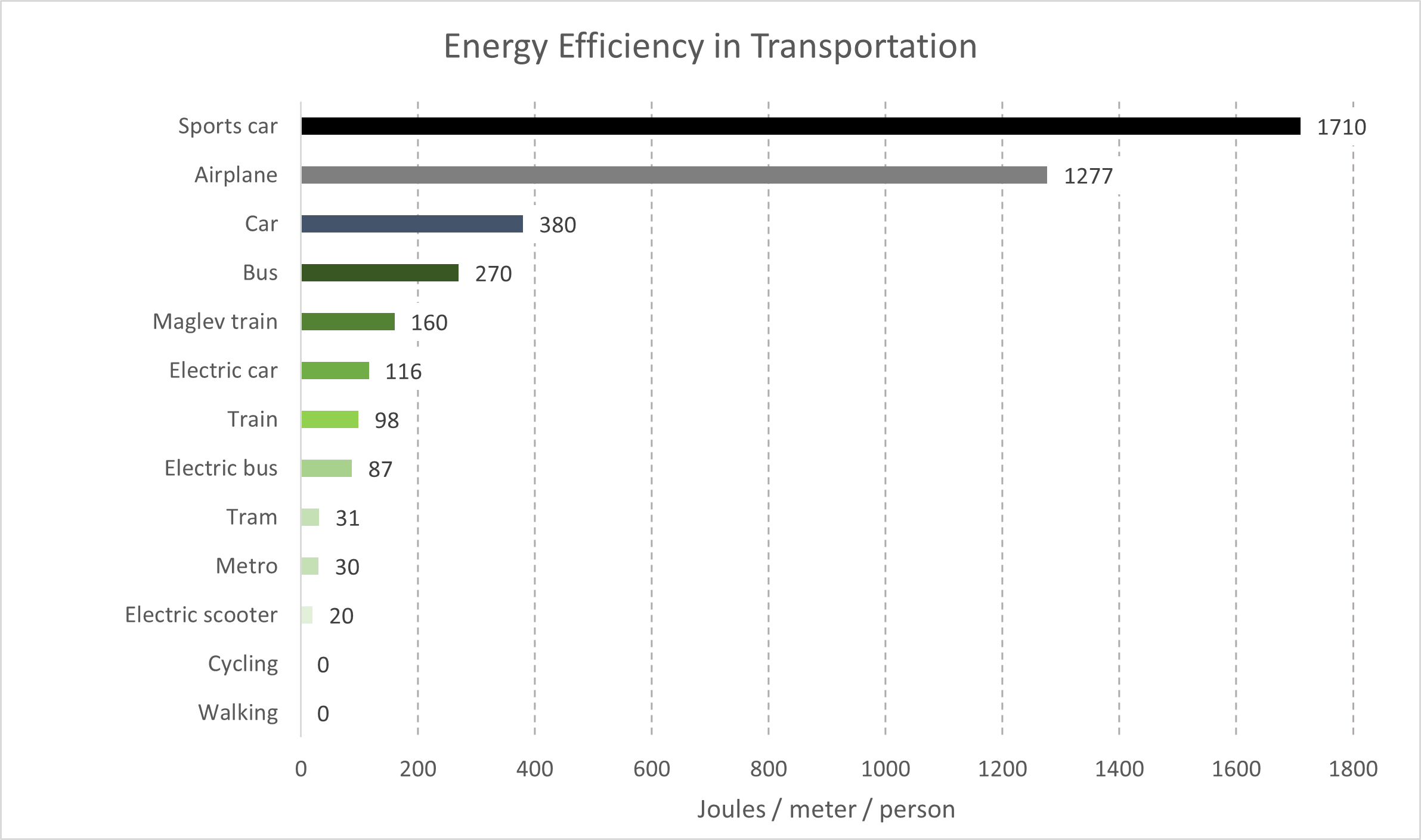
A horizontal bar chart showing modes of transportation from walking (0) to taking a commercial air flight (1277) showing the energy used per meter transported per person. — *Figure 1. Transportation energy-efficiency comparison*

In the case of object motion, in anything other than a vacuum, drag is proportional to the square of the speed of travel. Meaning it takes four times the force and energy to go twice as fast for a given distance. Movement of people and goods around our planet means traveling through either air or water (both are “fluids” in physics) and this concept helps explain why going faster requires much more energy.

Most transportation technologies operate on fossil fuels because, even now, the energy density of fossil fuels and the weight of the engines that run on them are difficult to rival. For example, nuclear energy technology presents challenges including waste, and specialized personnel required to operate safely, and weight, meaning nuclear-powered cars, buses, or airplanes are not happening anytime soon.

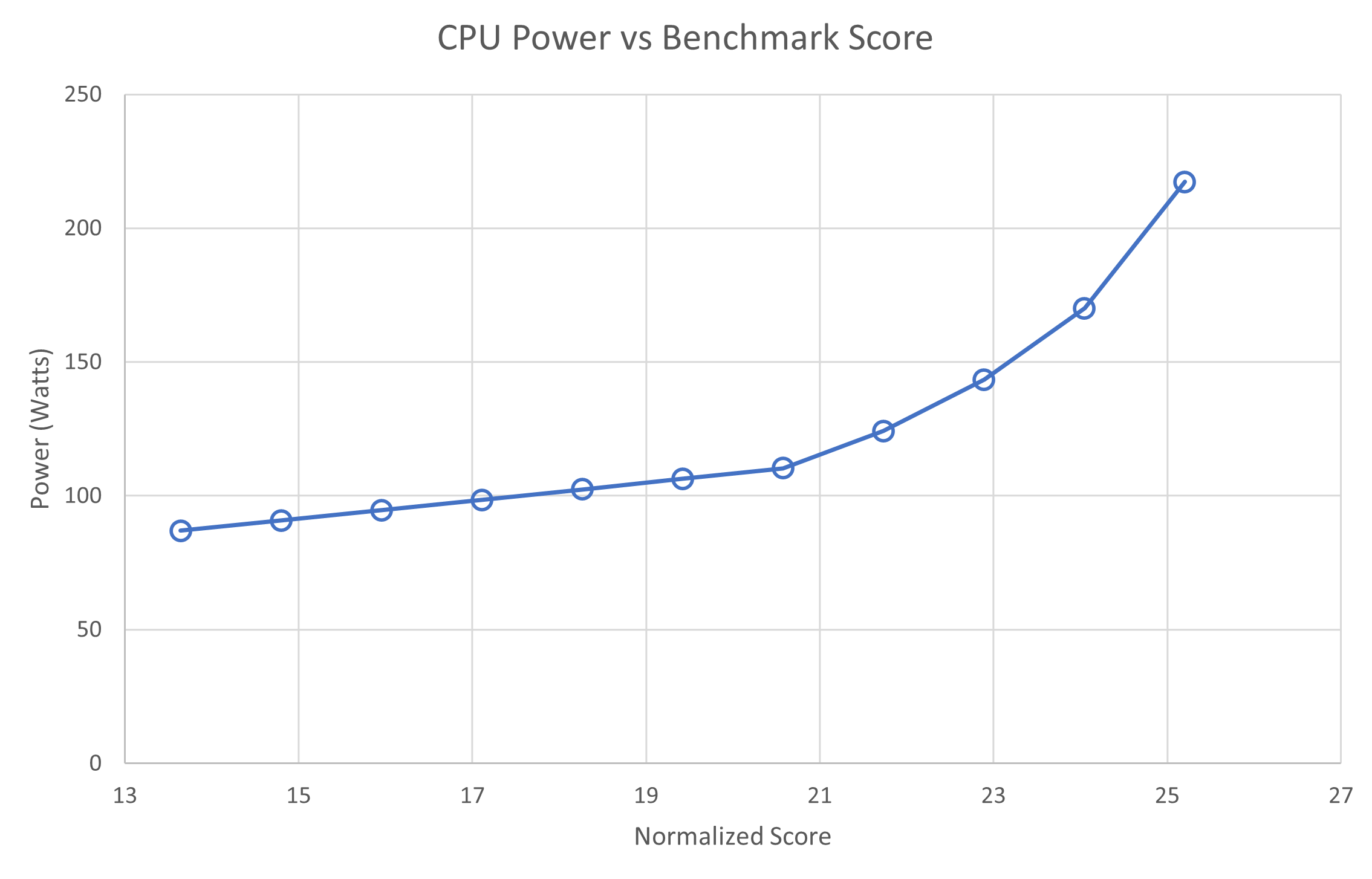
A line chart of Power compared to Integer speed showing that as speed increases, the power goes up, linearly at first, then exponentially. — *Figure 2. CPU power compared to a normalized benchmark score*

The silicon processor has the same kind of relationship with speed. The preceding chart shows that increasing integer processing speed is achieved with an increase in power (energy per unit time). So similar to transportation, the faster the processor goes, the more energy it uses.

You might be asking, “Why don’t computers run on tens of kilowatts today? They have been getting faster for 50 years.”

The answer is that as processors have gotten faster, they have also gotten smaller. Shrinking silicon features make them more efficient from an energy perspective, and therefore at constant power, can run faster at higher clock speeds. Loosely stated, this is known as Dennard scaling.

Multi-node parallel computing

A pivotal concept in HPC is the effect that parallel computing reduces wall-clock runtime at the expense of total aggregate compute time. For HPC applications containing small portions of serial operations (for the uninitiated, almost all do), the runtime asymptotically approaches the runtime of the serial operations as more computational resources are added.

This is known as Amdahl’s law.

This is important when considering the energy consumed by parallel computing. Assuming a compute unit draws the same amount of power while it performs a computation, means that a computational task will consume more power as it is parallelized among larger and larger sets of compute resources.

It means that a computational task will consume more power as it is parallelized among larger and larger sets of compute resources. Simultaneously, the task runs for less time. The hypothesis during this investigation is that the reduction in runtime by adding resources does not keep pace with the additional power required by incremental compute resources, and in the end uses more energy.

Or, as was discussed in the introduction, the faster you want to go, the more energy you will use.

Measuring energy usage

Using the Selene system, based on the NVIDIA DGX A100, engineers can collect various metrics, which are aggregated using Grafana. With its API, users can query power use over time for individual CPUs, GPUs, and power supply units, either for the whole job or a given time frame.

Using this data with timestamps from simulation output quantifies the energy used. The reported numbers for energy consumption do not take into account some factors:

Network switching infrastructure (network cards internal to servers are included)
Shared filesystem usage for data distribution and results collection
Conversion from AC to DC at the power supply
Cooling energy consumption for data center CRAC units

The largest of the errors is the item for an air-cooled data center and is closely aligned with the power usage effectiveness (PUE) for the data center (~1.4 for air-cooled and ~1.15 for liquid-cooled). Further, the AC to DC conversion could be approximated by increasing measured energy consumption by 12%. However, this discussion focuses on comparisons of energy, and both of these errors are ignored.

For the rest of this post, we use Watts (Joules per second) for power and kilowatt-hours (kWh) for energy.

Experiment setup

		Active NVIDIA Infiniband connections per node
		1	2	4
GPUs per node	1	✔
	2		✔
	4	✔	✔	✔

Table 1. Execution geometry of simulations

Due to various configurations of GPU-accelerated HPC systems worldwide, requirements, and stages of adoption for accelerated technologies across HPC simulation applications, it is useful to execute parallel simulations using different configurations of compute nodes. This optimizes performance and efficiency further.

The preceding table shows the five different ways that each application was scaled. The following plots use a consistent visual representation for ease of reading. Single NVIDIA InfiniBand connections use a dotted gray or black line. Dual Infiniband connections use a solid green line, and quadruple Infiniband connections use an orange-dashed line.

HPC application performance and energy

This section provides insights into some key HPC applications representing disciplines such as computational fluid dynamics, molecular dynamics, weather simulation, and quantum chromodynamics.

Applications and datasets

Application	Version	Dataset
FUN3D	14.0-d03712b	WB.C-30M
GROMACS	2023	STMV (h-bond)
ICON	2.6.5	QUBICC 10 km resolution
LAMMPS	develop_7ac70ce	Tersoff (85M atoms)
MILC	gauge-action-quda_16a2d47119	NERSC Large

Table 2. HPC simulation applications used for this study

FUN3D

FUN3D was first written in the 1980s to study algorithms and develop new methods for unstructured-grid fluid dynamic simulations for incompressible flow up to transonic flow regimes. Over the last 40 years, the project has blossomed into a suite of tools that cover not only analysis, but adjoint-based error estimation, mesh adaptation, and design optimization. It also handles flow regimes up to the hypersonic.

Currently, a US citizen-only code, research, academia, and industry users all take advantage of FUN3D today. For example, Boeing, Lockheed, Cessna, New Piper, and others have used the tools for applications such as high-lift, cruise performance, and studies of revolutionary concepts.

GROMACS

GROMACS is a molecular dynamics package that uses Newtonian equations of motion for systems with hundreds to millions of particles. It is primarily designed for biochemical molecules like proteins, lipids, and nucleic acids that have many complicated bonded interactions. GROMACS is extremely fast at calculating the non-bonded interactions (that usually dominate simulations) and many groups are also using it for research on non-biological systems (for example, polymers).

GROMACS supports all the usual algorithms from a modern molecular dynamics implementation.

ICON modeling framework

ICON modeling framework is a joint project between the Deutscher Wetterdienst (DWD) and the Max-Planck-Institute for Meteorology for developing a unified next-generation global numerical weather prediction (NWP) and climate modeling system. The ICON modeling framework became operational in DWD’s forecast system in January 2015.

ICON sets itself apart from other NWP tools through better conservation properties, with the obligatory requirement of exact local mass conservation and mass-consistent transport.

It recognizes that climate is a global issue, and therefore strives for better scalability on future massively parallel HPC architectures.

LAMMPS

LAMMPS is a classical molecular dynamics code. As the name implies, it is designed to run well on parallel machines.

Its focus is on materials modeling. As such, it contains potential models for solid-state materials (metals, semiconductors) soft matter (biomolecules, polymers), and coarse-grained or mesoscopic systems. LAMMPS achieves parallelism using message-passing techniques and a spatial decomposition of the simulation domain. Many of its models have versions that provide accelerated performance on both CPUs and GPUs.

MILC

MILC is a collaborative project used and maintained by scientists studying the theory of strong interactions of subatomic physics, otherwise called quantum chromodynamics (QCD). MILC performs simulations of four-dimensional SU(3) lattice gauge theory on MIMD parallel machines. MILC is publicly available for research purposes, and publications of work using MILC or derivatives of this code should acknowledge this use.

Parallel scalability

In the following plots, we show a dimensionless quantity SPEEDUP, or strong scaling, as calculated in the standard fashion:

$SPEEDUP = \frac{runtime_{1\ GPU \ and\ 1\ IB}}{runtime_{n\ GPUs\ and\ m\ IB}}=0$

Parallel SPEEDUP is often plotted against an “ideal” SPEEDUP, where employing one computational resource gives a SPEEDUP value of one, employing two resource units gives a SPEEDUP value of two, and so on. This is not done here because multiple scaling traces are being shown, and the plots get very crowded with data when each has its own ideal SPEEDUP reference.

The number of GPUs per node and the number of enabled CX6 EDR Infiniband connections for each node sweep are shown in the legend with {# GPUs / node} – {# IB / node}.

Left side: FUN3D Speedup showing GPU per node and IB connections per node perform the same starting with one GPU and diverge slightly when scaled out to 128 GPUs with the 2-2 configuration being the most performant, and the max performance point at 64 GPUs. — *Figure 3. FUN3D Speedup with FUN3D plotted relative to four GPUs each with one active GPU and InfiniBand connection*

GROMACS speedup showing the 4-1 configuration being a poor choice, and both the 2-2 and 4-4 configurations scaling very well. — *Figure 4. GROMACS speedup plotted relative to one GPU with and a single node with one InfiniBand connection*

Figure 5. ICON Speedup with ICON plotted relative to 64 GPUs with one GPU and one active InfiniBand connection

All LAMMPS configurations scaling almost identically except 4-1 is 20% worse. — *Figure 6. LAMMPS *Speedup* with LAMMPS plotted relative to eight GPUs with one GPU and one active InfiniBand connection*

MILC speedup scaled from 32 to 256 GPUs where 4-2 and 4-4 configurations scale the best and reach the highest performance. — *Figure 7. MILC Speedup plotted relative to 32 nodes with one GPU and one active InfiniBand connection*

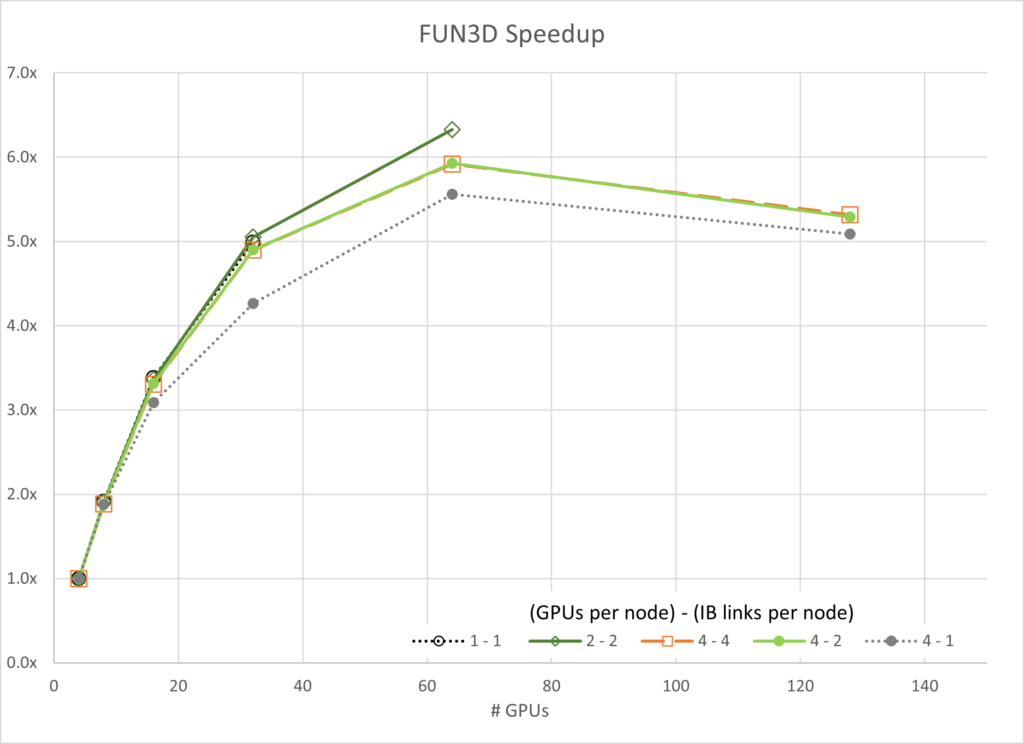
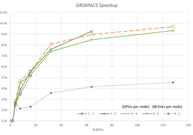
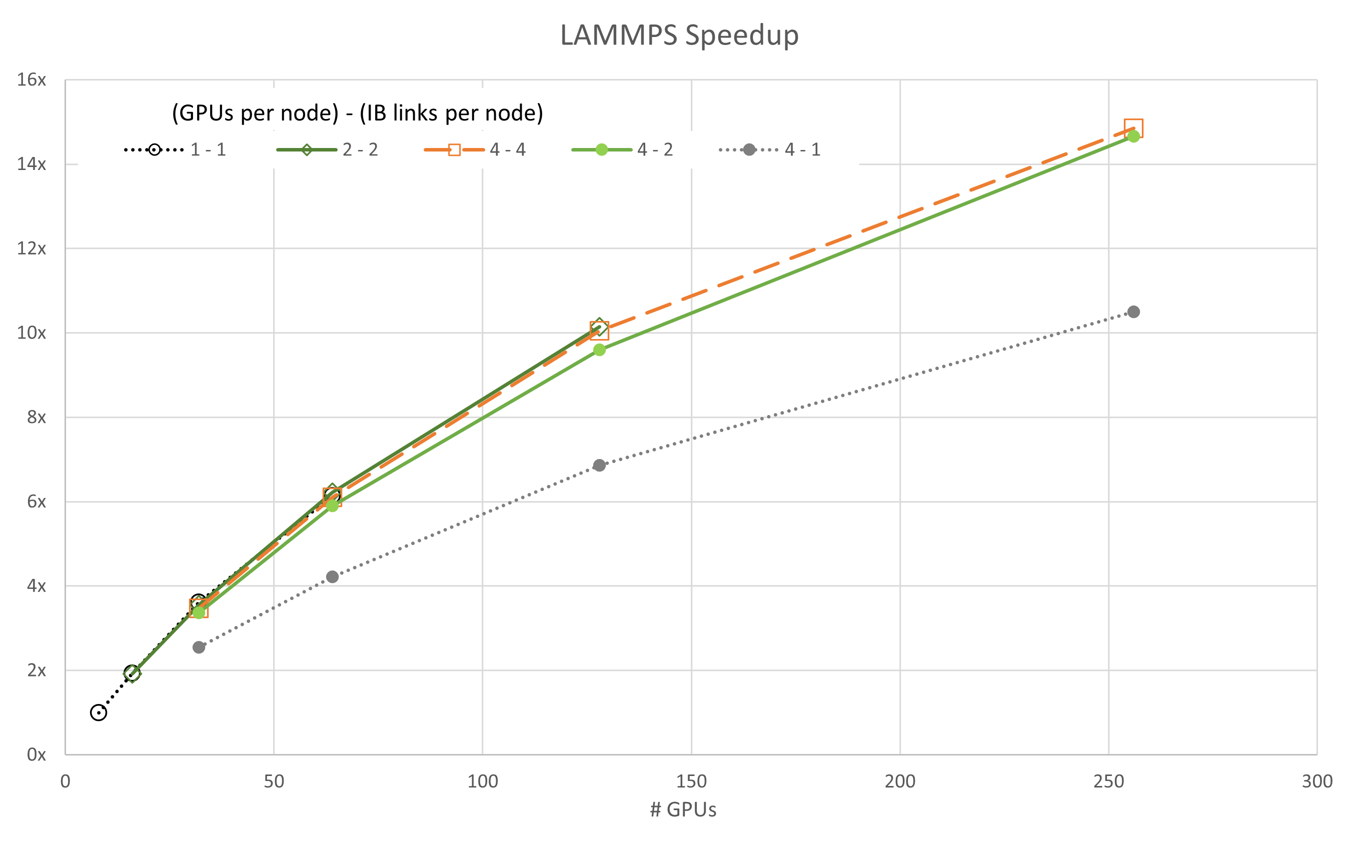
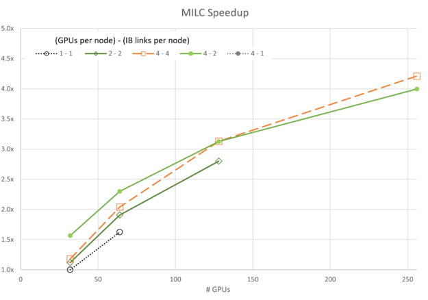
Figures 3 through 7 show the scalability of each of the simulations. Generally, most of the data follows the trend expected based on Amdahl’s law. A notable exception is the GROMACS configuration using four GPUs and one InfiniBand connection per node (labeled 4-1). This configuration exhibits negative scaling at first, meaning it slows down as resources are added before it starts to scale.

Given the network configuration, it seems that ‌scaling is bound by the bandwidth of the network and the data each parallel thread is trying to communicate. As the number of resources grows between 16 and 32 GPUs, the task reaches a point where it is no longer bandwidth-bound and scales to a small degree.

Similar outlier behavior for the 4-1 configuration is seen for ICON and LAMMPS, though both scale much more readily than GROMACS.

It is also interesting to note that the 4-4 configuration is not always the best for performance. For FUN3D (2-2) and a portion of the MILC (4-2), scaling other configurations shows superior performance by small margins. However, in all cases, the 4-4 configuration is among the best configurations.

Energy Usage

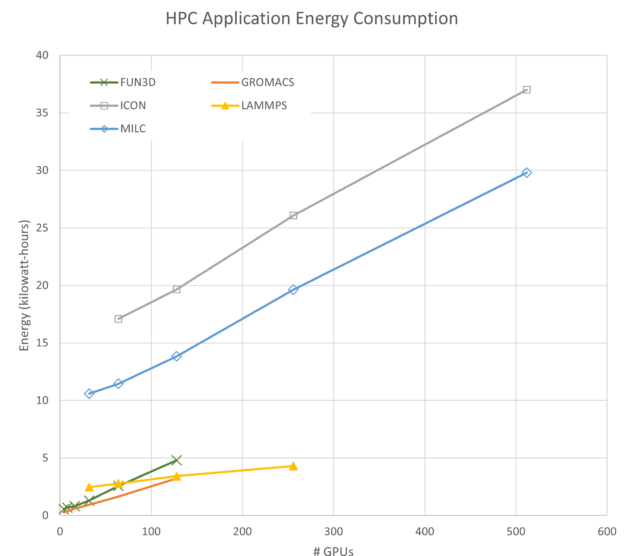
ICON uses the most energy, ranging from 17–37 kWh, linearly growing as it scales. MILC's energy consumption has the same shape but ranges between 10 and 30 kWh. FUN3D, LAMMPS, and GROMACS all use less than 5 kWh, and slope up to the right, with LAMMPS being the flattest, ranging between 2.5 and 4 kWh on 16-256 GPUs. — *Figure 8. Energy usage for HPC applications running with four GPUs and four Infiniband connections per node*

For brevity, Figure 8 shows only the four GPU and four IB connections (4-4) energy consumption in a single plot. The amount of energy used by each simulation is arbitrary and can be adjusted up or down by changing the problem size or analysis type. There are two relevant characteristics to note:

The slope for each application is positive, meaning that they use more energy as they scale.
Some applications like FUN3D increase used energy quickly, while others like LAMMPS increase more gradually.

Time to solution compared to energy to solution

Some may conclude from Figure 8 that the best configuration to run these simulations is by minimizing the number of resources used per simulation. While the conclusion from an energy standpoint is correct, there are more objectives to consider beyond energy.

For example, in the case of a researcher working against a project deadline, time to solution is crucially important. Or, in the case of a commercial enterprise, final data is often required to start the manufacturing process and get a product ready for release to market. Here, too, the time to solution value may outweigh the extra energy required to produce the simulation output sooner.

Therefore, this is a multi-objective optimization problem with several solutions depending on the weights of each defined objective.

The ideal case

Before exploring the objectives, consider the following ideal case:

A perfectly parallel (meaning no serialized operations) accelerated HPC application, which scales linearly as additional processors are added. Graphically, the SPEEDUP curve is simply a line starting from (1,1) and going up and to the right at a slope of 1.0.

For such an application, now consider energy. If every processor added consumes the same amount of power, then power consumption during the run is the following equation:

$Power = n \times P_1$

In this case, $n$ is the number of processors used and $P_1$ is the power used by one GPU.

$Energy = Power \times time$

But time is an inverse function of $n$ , so you can rewrite it as follows:

$Energy = P_1 \times time_1$

The $n$ values cancel, and we see that $Energy$ , in the ideal case, is not a function of the number of GPUs and is in fact constant.

$Energy= n \times P_1 \times \frac{time_1}{n}$

In several cases, HPC applications are not ideal in either parallel speedup or energy. Because speedup is a case of diminishing returns as resources are added, and energy grows roughly linearly as resources are added, there should be a number of GPUs where the ratio of speedup to energy is a maximum.

More formally, assuming equal weights for energy and time:

$SPEEDUP_{Energy} = \frac{SPEEDUP}{EnergyRatio} = \frac{\left [ \frac{runtime_{1\ GPU \ and\ 1\ IB}}{runtime_{n\ GPUs\ and\ m\ IB}} \right ]}{\left [ \frac{energy_{n\ GPUs\ and\ m\ IB}}{energy_{1\ GPUs\ and\ 1\ IB}} \right ]}\\ = \left [ \frac{runtime_{1\ GPU \ and\ 1\ IB}}{runtime_{n\ GPUs\ and\ m\ IB}} \right ] \times \left [ \frac{energy_{n\ GPUs\ and\ m\ IB}}{energy_{1\ GPUs\ and\ 1\ IB}} \right ]$

In this formula, the following is constant:

$\left [ runtime_{1\ GPU \ and\ 1\ IB} \times energy_{1\ GPU \ and\ 1\ IB}\right ]$

You should maximize the following:

$\frac{1}{\left [ runtime_{n\ GPU \ and\ m\ IB} \times energy_{n\ GPU \ and\ m\ IB}\right ]}$

Or, you should minimize the following:

$runtime_{n\ GPU \ and\ m\ IB} \times energy_{n\ GPU \ and\ m\ IB}$

If one plots runtime on one axis and energy on the opposite axis, then the quantity to minimize is simply the area defined by runtime multiplied by energy.

Defining the problem this way also enables the exploration of multiple independent variables, including but not limited to the number of resources used in a parallel run, GPU clock frequency, network latency, bandwidth, and any other variable that influences runtime and energy usage.

Balanced speed and energy

The following plots are the product of runtime and energy consumption, where the independent variable is the number of GPUs in the parallel run. These plots provide one method to determine one solution among the Pareto front of solutions for optimization of runtime and energy.

A curved plot showing decreasing then increasing with a minimum at 16 GPUs. The 4-2 and 4-4 configurations are best {right side}. — *Figure 9. Runtime * Energy for FUN3D showing a minimum of 16-32 GPUs*

A less obvious optimum for GROMACS with 2-2 being almost flat between four and 32 GPUs and 4-2 and 4-4 configurations best with the peak at eight GPUs. — *Figure 10. Runtime * Energy for GROMACS*

Figure 11. Runtime * Energy for ICON

LAMMPS decreases Runtime * Energy throughout the 8-256 GPU range. 4-4 and 4-2 configurations are best. — *Figure 12. Runtime * Energy for LAMMPS*

MILC shows a clear minimum at 32 GPUs using 4-4 configuration. — *Figure 13. Runtime * Energy for MILC*

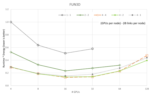
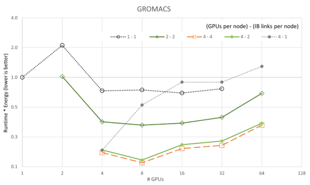
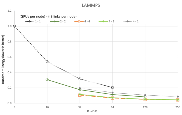
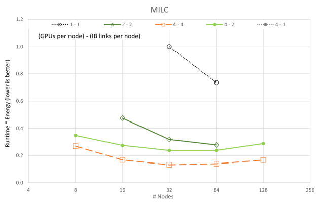
The preceding figures show changes in Runtime * Energy as each of the five applications and five GPU/network configurations are scaled with GPU count. Different from the scalability plots of performance, we see that in all cases the 4-4 configuration (reminder, “4-4” refers to {# GPUs / node} – {# IB / node}) is the best with the 4-2 configuration occasionally a close second. Aligned with the scalability plots, the 1-1 configuration is consistently the worst configuration, likely because of overhead on each server being mostly idle (that is each node had eight A100 GPUs, and eight CX6 Infiniband adaptors).

Perhaps more interesting is the fact that both LAMMPS and ICON show they have not reached a minimum in Runtime * Energy for the data we collected. Larger runs should be performed for LAMMPS and ICON to show minima.

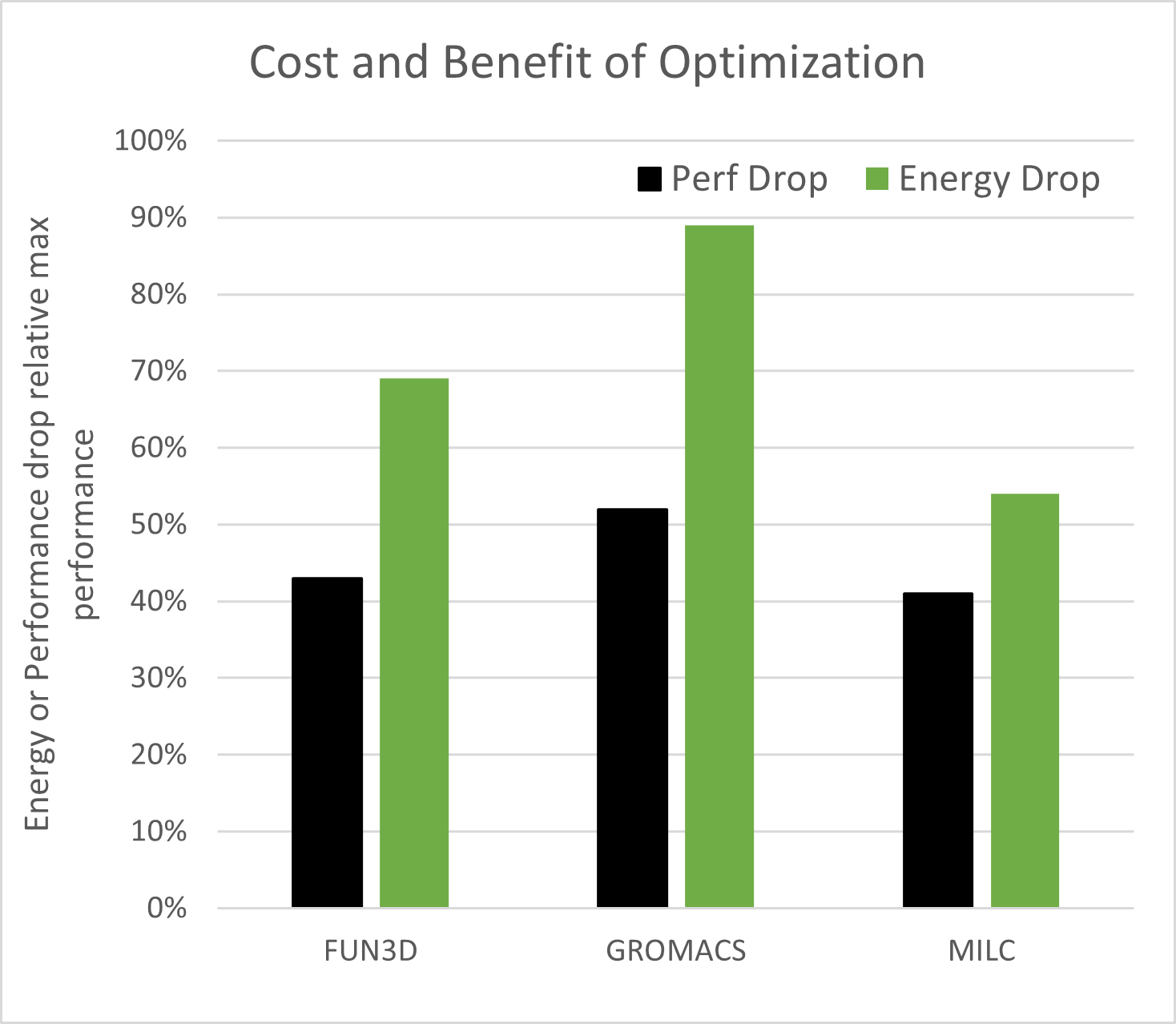
A graph showing energy performance and energy drop. — *Figure 14. Cost and benefits of optimizing time to solution and energy to solution compared to maximum performance*

The desired outcome of the optimization is to run simulations at increased efficiency. Comparing the performance drop to the energy drop per simulation (normalized by the maximum performance point) is a simple way to check that the optimization output achieved efficiency increase. If the performance drop is less than the energy drop, the efficiency is higher, which is seen for FUN3D, GROMACS, and MILC in Figure 14.

There is an opportunity for saving energy and the performance cost compared to the maximum performance point. This is shown in Figure 14. ICON and LAMMPS were not plotted because they did not display a minimum point in the optimization. The desired outcome is that performance drops less than the energy used per simulation, and that is precisely what is seen for FUN3D, GROMACS, and MILC.

Navigating the intersection of multi-node scalability and energy

Data center growth and the expanding exploration and use of AI will drive increased demand for data centers, data center space, cooling, and electrical energy. Given the fraction of electricity generated from fossil fuels, greenhouse gasses driven by data center energy demands are a problem that must be managed.

NVIDIA continues to focus on making internal changes and influencing the design of future products, maximizing the positive impact of the AI revolution on society. By using the NVIDIA accelerated computing platform, researchers get more science done per unit of time and use less energy for each scientific result. Such energy savings can be equated to a proportional amount of carbon dioxide emissions avoided, which benefits everyone on the planet.

Read the recent post, Optimize Energy Efficiency of Multi-Node VASP Simulations with NVIDIA Magnum IO for a deeper dive focused on VASP and energy efficiency.

This short discussion and set of results are offered to jump-start a conversation about shifting the way HPC centers allocate and track resources provided to the research community. It may also influence users to consider the impact of their choices when running large parallel simulations, and the downstream effects.

It is time to start a conversation regarding energy to solution for HPC and AI simulations and the multi-objective optimization balance with time to solution discussed here. Someday, the HPC community may measure scientific advancements per megawatt-hour, or perhaps even per mTon CO2eq, but that won’t be achieved until conversations begin.

For more information, visit NVIDIA sustainable computing. Read about NERSC and their impressions of the accelerated platform. Or, listen to Alan Gray’s NVIDIA 2023 GTC session about tuning the accelerated platform for maximum efficiency.

Energy Efficiency in High-Performance Computing: Balancing Speed and Sustainability

Multi-node parallel computing