
This post is part of a series about optimizing end-to-end AI.
While NVIDIA hardware can process the individual operations that constitute a neural network incredibly fast, it is important to ensure that you are using the tools correctly. Using the respective tools such as ONNX Runtime or TensorRT out of the box with ONNX usually gives you good performance, but why settle for good performance when you can have great performance?
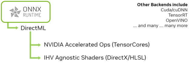
In this post, I discuss a common scenario, ONNX Runtime with the DirectML backend. These are the two main components from which WinML is constructed. When used outside of WinML they can offer greatly increased flexibility in terms of support for operator sets, as well as supporting backends other than DML, like TensorRT.
To get the great performance out of ONNX Runtime and DML, it is usually worthwhile going beyond a basic implementation. Start with a common scenario when using ONNX Runtime.
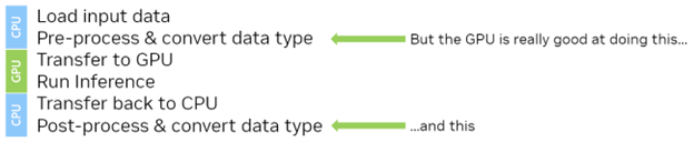
- Some image data is loaded from disk.
- The int8 image data is preprocessed in some way, such as scaled and converted to float16.
- The image data is loaded onto the GPU.
- Inference is run on the image data.
- The results are loaded back to the CPU.
- The results are post-processed or perhaps sent to another model.
There are several issues here. If you use ONNX Runtime from scratch, you supply pointers to data in system (CPU) memory. ONNX Runtime transfers the data to and from the GPU when you run inference by calling Ort::Session::Run(...) and transferring the data back to system (CPU) memory when inference is complete.
While this sounds convenient from an implementation point of view, you may have a pre-process stage before inference and a post-process stage after inference. With this current workflow, you must either pre– and post-process the data on the CPU or have a roundtrip to the GPU and back before ONNX Runtime transfers everything back to the GPU a second time for inference.
A much better way would be to load your original data to the GPU, either in its entirety or in tiles first, perform the preprocessing step on the GPU (more on this shortly), and leave it on the GPU ready for inference. This way, you have leveraged the massively parallel power of the GPU to perform your pre-processing step and have reduced the size of the initial transfer as you are now transferring int8 data and not float16 data.
That’s all well and good in theory, but how do you put that into practice using ONNX Runtime and DirectML? For that, you must delve into DirectX 12, upon which DirectML is built.
For more information about the implementations that I discuss in this post, see the code example and comments.
DirectX12
DirectX 12 may be somewhat verbose when compared to OpenGL and CUDA. For rendering graphics, there can be a lot of pipeline state to manage. You only have to use the compute pipeline, which is much simpler. In any case, DirectX 12, like any other API or SDK, has a learning curve but it is neither steep nor lengthy.
DirectX12 enables fast and highly configurable access to the GPU by exposing lower-level constructs that you can use to control when and how you schedule work on the GPU. ONNX Runtime with DML already uses it, but you want to gain access to those same resources that ONNX and DML are using so that you can use them to perform the preprocessing and transfers.
DirectX 12 exposes hardware constructs called command queues. You can record commands into these queues on the CPU and send them to the GPU to be dispatched. These commands can be run multiple times without being re-recorded. By creating multiple queues, you can perform more than one job in parallel on the GPU. It is often the case that a single inference may not actually saturate the processors on the GPU and you may be able to do more than one thing at the same time. More on this later.
Here’s a high-level view of such a DirectX 12 workflow:
- Get a reference to the graphics card (the adapter).
- Create a logical reference to the graphics device. You use this to allocate memory and issue commands.
- Get a reference to a command queue, from the device.
- Write your compute shaders for preprocessing, which is simpler than you might think.
- Create a compute pipeline state object.
- Allocate some memory on the device for inputs and outputs. You can transfer to and from this memory at any time.
- Add commands to the command queue.
- Execute the queue.
The queue that you create is the same queue that ONNX Runtime gives to DirectML. You can build your new high-performance features as an extension of what ONNX Runtime already gives you.
What you are about to learn applies to ONNX and DirectML, as well as many other compute tasks.
Get a reference to the graphics card
Depending on the type of system that you have, you may have one graphics card, many graphics cards, or no graphics card at all.
The first thing to do is to query the system to discover what you can play with. This enables you to acquire an interface to the actual physical device through Direct X Graphics Interface (DXGI). From this physical device interface, you can create a reference to a logical device that gives you access to the device memory and command queues that DirectX needs for running.
There are several types of command queues available for different tasks, such as rendering, copying, and compute work. It is possible to perform some tasks in parallel to each other, such as copy and compute work. For more information, see the code example.
Setting up ONNX Runtime
To use ONNX Runtime with DirectML in this project, first set up the reference to the logical device. Then, create a reference to a DML device using the logical DirectX12 device. You also create a queue for DML to use. Then, when you create the session options structure for the DML execution provider, you use the extended form to create the ORT session using the DirectX12 constructs that you created earlier.
	Ort::SessionOptions opts;
	OrtSessionOptionsAppendExecutionProviderEx_DML(
opts, m_dml_device.Get(),
m_copy_queue->GetD3D12CmdQueue().Get())
You can now create the session in the normal way using the SessionOptions object.
With the session created, you can now turn to initializing the resources to pass input data to the model and receive output data from the model. To do that, you query the model for the tensor shapes and formats that it expects.
Memory and memory transfers
If you were to use ONNX Runtime from a basic implementation, the input and output data would start out in CPU memory and ONNX Runtime would manage the transfers to and from the GPU. In simple cases, such as when inference is performed on an image in its entirety, this is probably fine.
However, in practice, most large images are broken up into tiles, perhaps with some overlap and processed in sequence. In situations such as this, a considerable performance gain can be achieved by managing the transfers yourself.
- You can control when your transfers take place.
- You can perform transfers in parallel with other compute work.
The memory interface of DirectX 12 is flexible and can be used in a variety of ways to perform transfers. The method that gives you the most granularity with respect to performing data transfer is to stage memory yourself.
- Create a dedicated queue for staging memory:
- type : D3D12_COMMAND_LIST_TYPE_COPY
- Create two ID3D12Resource objects:
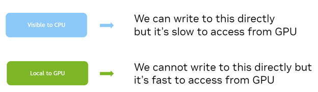
- D3D12_HEAP_TYPE_UPLOAD: Visible from the host.
- D3D12_HEAP_TYPE_DEFAULT: Local to the GPU.
- Use either committed or placed resources:
- Committed resource: DX12 creates and manages the heap for you.
- Placed resource: You provide the heap. Use for suballocation.
- Create a command list and dispatch a copy command. This performs the copy from the host to the device.
After you have your data on the GPU, create a view object to refer to it and an Ort Value object with a binding to this memory. However, you do not feed your raw transferred data into the model as it stands, as there is still one more important step to perform.
Faster preprocessing
Now you have control over when and how the data is transferred to and from the GPU. You can now look at how to move the pre– and post-processing to the GPU as well.
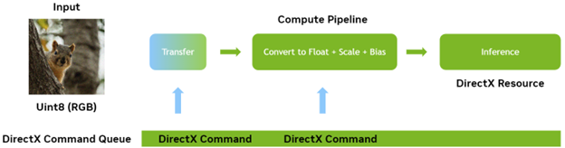
It is common in most computer vision applications for some input to be provided in an integer format, such as RGB8, and convert this to a scaled and biased floating-point representation.
If you are using ONNX Runtime with DML out-of-the-box, it is hard to do this on the GPU because the data starts and ends its journey on the CPU. Now, you can perform these transfers yourself and so you have control over the lifecycle of the memory. You can also move this pre– and post-processing to a custom compute pass and run it as a part of your end-to-end inference pipeline.
What you must do is insert a compute step after the transfer to the GPU but before you run inference. The compute step in this case takes the RGB8 integer data that you transferred to the GPU and pass this to a compute kernel (shader) that performs the scaling and bias. While it does this, it also converts the data to floating point in the precision required by the model. For the best performance this should be FP16.
All the actions that you must perform on the data are in-place actions in that each pixel in the input has the same action performed on it and there is no dependency on any of its neighbors. This type of work is easy to perform in parallel so it is an excellent candidate to leverage the power of the GPU.
To run a compute shader using DirectX 12, create what’s called a pipeline state object. For graphics rendering, this can be quite an involved process but for compute processing, it’s considerably simpler.
A pipeline state object essentially precompiles all the state needed to do some work on the GPU including the shader bytecode that runs and the bindings to the resources to be used.
You first create an object called a root signature, which is similar to a function signature in that it describes the attributes and output of the pipeline. You can then use this root signature to create the pipeline state object itself providing the actual buffer bindings for input and output.
After the pipeline is created, create a command buffer and record the necessary command to run the compute shader. For more information, see the code example.
Synchronization and leveraging more parallelism
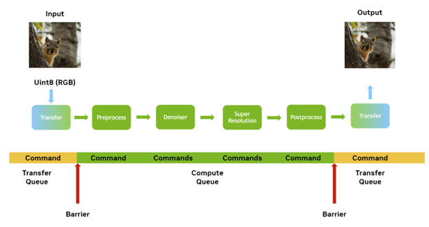
NVIDIA hardware can do some different tasks in parallel, significantly performing transfers to and from the GPU in parallel with any compute work being performed. When the DML model is executing on the GPU, it is compute work.
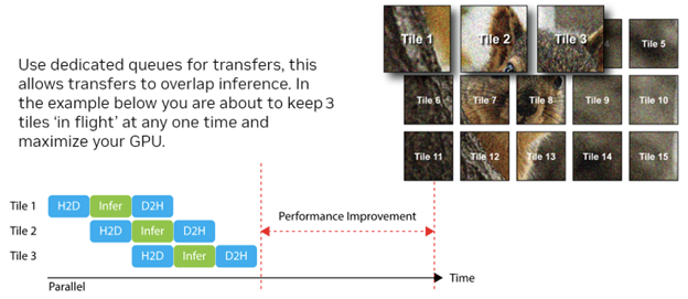
I recommend that you set up your end-to-end pipeline such that one lot of inference work, for example, a tile, can be performing inference while the next lot of inference work is being transferred to the GPU so that it can run next. In fact, it is even possible to run the actual compute or inference part of more than one tile in parallel if there are enough resources available on the GPU.
For these overlaps in processing to take place, the compute or transfer work must be performed in their own queues, some of which can run in parallel to each other. This raises the important concept of synchronization. If you have transfer running in one queue of some data on which you run inference on another queue, then you must ensure that the data has finished transferring by the time you have to run any compute or inference steps.
Synchronization can be performed in several ways from both the CPU side and the GPU side, however you want as little interaction from the CPU as possible. Use a resource barrier. This causes the queue to wait until the conditions set by the barrier have been met. You use two barriers:
Resource transition barrier
Remember that you are transferring the data from the host to the device. At the time that you transfer the data, the destination buffer is in a state where data can be transferred to it from the CPU. This may not be the most optimal state for it to be in when bound to the pipeline, so you have to provide a transition.
The requirement for this is dependent on the hardware platform, but the transition is needed for the use of DirectX12 to be valid.
UAV barrier
This type of barrier simply blocks the queue until all the data has finished transferring. By using a barrier in this way, you enable the GPU to wait without the CPU getting involved at all and improving performance.
CD3DX12_RESOURCE_BARRIER barrier2 = CD3DX12_RESOURCE_BARRIER::UAV(
		m_ort_input_buffer->GetD3DResource().Get()
	);
After the two barriers are created, add them to the command list in one step.
CD3DX12_RESOURCE_BARRIER barriers[2]  = {barrier1, barrier2};
m_cmd_list_stage_input->ResourceBarrier(2, barriers);
You can now put all the pieces together. You have seen that you can create and manage not only the resources that you can use to dispatch the transfer and compute work but also the time at which they are dispatched.
Now you just need the two queues:
- Transfer queue: Used to dispatch the transfer commands.
- Compute queue: Used to dispatch both the pre– and post-processing commands and the actual ONNX runtime session itself.
You also need a command list for each to record commands into.
There must be some synchronization between the transfer and the compute to ensure that the transfers have completed before the work on the data being transferred commences. There’s an opportunity to optimize here.
NVIDIA hardware is all about parallelism and it can do things such as perform transfers and compute work at the same time. When you deal with a single job, then there is little opportunity to overlap the transfer with compute, as you must wait for the transfer to complete before the compute starts.
Typically, in the case of an image-processing job, you split the work up into tiles. For large images, it’s likely that there isn’t enough device memory to perform the work in a single run. Use this parallelism by treating each tile as a series of tasks to be performed. You can then put several tiles ‘in flight’ at any one time, with a synchronization point between each critical stage:
- First tile: Copying data back to CPU memory.
- Second tile: Running inference and compute work.
- Third tile: Copying data to GPU memory.
All three tasks can happen in parallel. There may even be cases where more than one tile of compute work can take place with a certain degree of overlap if it does not saturate the GPU.
Conclusion
I covered a lot in this post. The only way to get a practical understanding of the mechanics of these approaches is by doing. I encourage you to spend time experimenting with the example code, which uses ONNX models exported from NVIDIA DL Designer.
For more information about what is taking place during execution, see the code comments.
