
This post is the third in a series about optimizing end-to-end AI.
When your model has been converted to the ONNX format, there are several ways to deploy it, each with advantages and drawbacks.
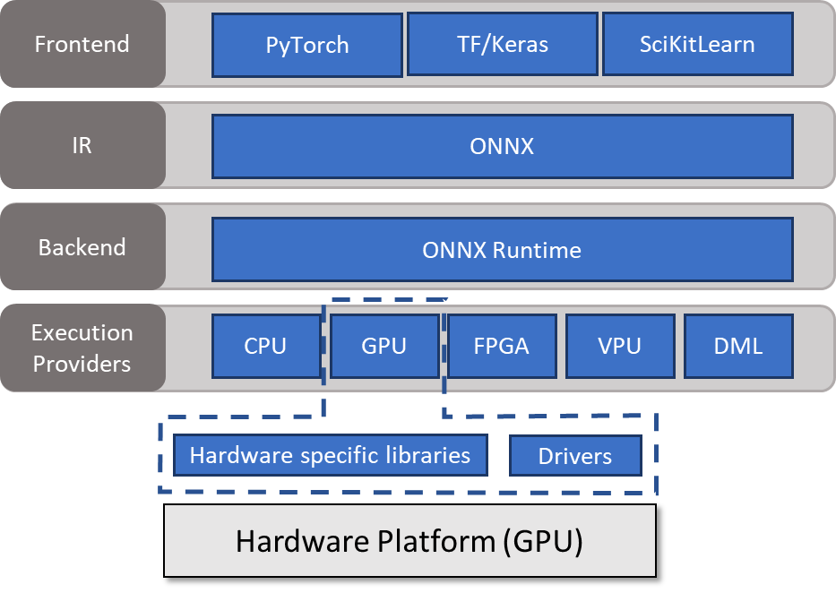
One method is to use ONNX Runtime. ONNX Runtime serves as the backend, reading a model from an intermediate representation (ONNX), handling the inference session, and scheduling execution on an execution provider capable of calling hardware-specific libraries. For more information, see Execution Providers.
In this post, I discuss how to use ONNX Runtime at a high level. I also go into more depth about how to optimize your models.
Run a model with ONNX Runtime
ONNX Runtime is compatible with most programming languages. As in the other post, this post uses Python for simplicity and readability. These examples are just meant to introduce the key ideas. For more information about the libraries for all popular operating systems, programming languages, and execution providers, see ONNX Runtime.
To infer a model with ONNX Runtime, you must create an object of the InferenceSession class. This object is responsible for allocating buffers and performing the actual inference. Pass the loaded model and a list of execution providers to use to the constructor. In this example, I opted for the CUDA execution provider.
import onnxruntime as rt

# Create a session with CUDA and CPU ep
session = rt.InferenceSession(model,
                              providers=['CUDAExecutionProvider',
                                         'CPUExecutionProvider']
					)
You can define session and provider options. ONNX Runtime’s global behavior can be modified using session options for logging, profiling, memory strategies, and graph parameters. For more information about all available flags, see SessionOptions.
The following code example sets the logging level to verbose:
# Session Options
import onnxruntime as rt
options = rt.SessionOptions()
options.log_severity_level = 0

# Create a session with CUDA and CPU ep
session = rt.InferenceSession(model,
                              providers=['CUDAExecutionProvider',
                                         'CPUExecutionProvider'],
															sess_options = options
					)
Use provider options to change the behavior of the execution provider that has been chosen for inference. For more information, see ONNX Runtime Execution Providers.
You can also obtain the available options by executing get_provider_options on your newly created session:
provider_options = session.get_provider_options()
print(provider_options)
Run the model
After you build a session, you must generate input data that you can then bind to ONNX Runtime. Following that, you can invoke run on the session, passing it a list of output names as well as a dictionary containing the input names as keys and ONNX Runtime bindings as values.
# Generate data and bind to ONNX Runtime
input_np = np.random.rand((1,3,256,256))
input_ort = rt.OrtValue.ortvalue_from_numpy(input_np)

# Run model
results = session.run(["output"], {"input": input_ort})
ONNX Runtime always places inputs and outputs on the CPU by default. As a result, buffers are constantly copied between the host and device, which you should avoid as much as possible. It is feasible to use and reuse device-generated buffers.
Model optimizations
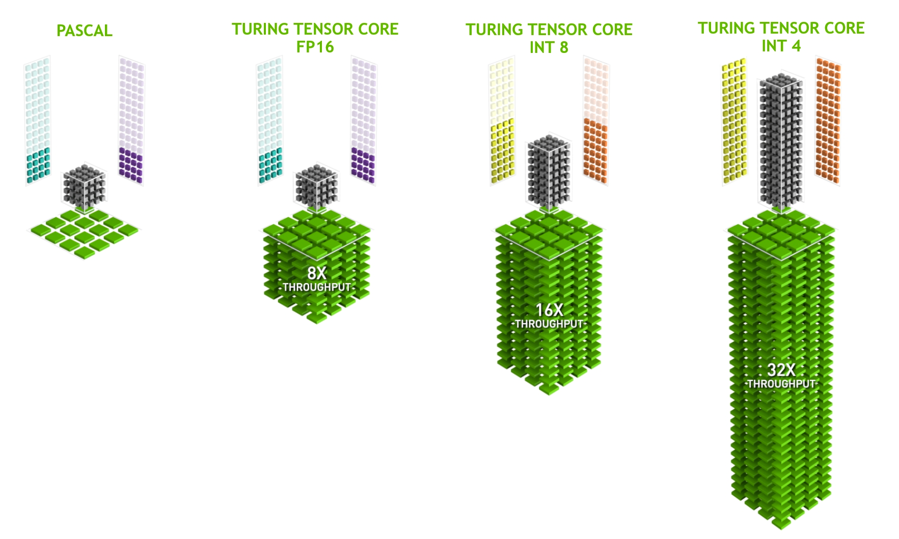
To get the most performance out of inference, I recommend that you make use of hardware-specific accelerators: Tensor Cores.
On NVIDIA RTX hardware, from the NVIDIA Volta architecture (compute capability 7.0+) forward, the GPU includes Tensor Cores to accelerate some of the heavy-lift operations involved with deep learning.
Essentially, Tensor Cores enable an operation called warp matrix multiply-accumulate (WMMA), providing optimized paths for FP16-based (HMMA) and integer-based multiply-accumulate (IMMA).
Precision conversion
The first step in using Tensor Cores is to export the model to a lower precision of FP16 or INT8. In most circumstances, INT8 provides the best performance, but it has two drawbacks:
- You must recalibrate or quantize weights.
- The precision may be worse.
The second point depends on your application. However, when working with INT8 input and output data such as photos, the consequences are often negligible.
On the other hand, FP16 does not require recalibration of the weights. In most cases, it achieves similar accuracy as FP32. To convert a given ONNX model to FP16, use the onnx_converter_common toolbox.
import onnx
from onnxconverter_common.float16 import convert_float_to_float16

model_fp32 = onnx.load("model.onnx")
model_fp16 = convert_float_to_float16(copy.deepcopy(model_fp32))
onnx.save(model_fp16, "model_fp16.onnx")
If the weight in the original model exceeds the dynamic range of FP16, there will be overflow. Any unwanted behavior can be overcome by using the auto-mixed precision (amp) exporter. This converts the model’s Ops to FP16 one by one, checking its accuracy after each change to ensure that the deltas are within a predefined tolerance. Otherwise, the Op is kept in FP32.
You need two more things for this type of conversion:
- An input feed dictionary containing the input names as keys and data as values. It is important that the data provided is in the right data range, though it is best if actual inference data is used.
- A validation function to compare if the results are in an acceptable error margin. In this case, I implemented a simple function that returns true if two arrays are element-wise equal within a tolerance.
import onnx
import numpy as np
from onnxconverter_common.auto_mixed_precision import auto_convert_mixed_precision

# Could also use rtol/atol attributes directly instead of this
def validate(res1, res2):
    for r1, r2 in zip(res1, res2):
        if not np.allclose(r1, r2, rtol=0.01, atol=0.001):
            return False
    return True

model_fp32 = onnx.load("model.onnx")
feed_dict = {"input": 2*np.random.rand(1, 3, 128, 128).astype(np.float32)-1.0}
model_amp = auto_convert_mixed_precision(model_fp32, feed_dict, validate)
onnx.save(model_amp, "model_amp.onnx")
During the conversion from FP32 to FP16, there are still possible problems apart from the dynamic range. It can happen that unnecessary or unwanted cast operations are inserted into the model. You must check this manually.
Architecture considerations
The data and weights must be in the correct layout. Tensor Cores consume data in NHWC format. As I mentioned earlier, ONNX only supports the NCHW format. However, this is not an issue as the backends insert conversion kernels before Tensor Core–eligible operations.
Having the backend handle the layout can result in performance penalties. Because not all operations support the NHWC format, there might be multiple NCHW-NHWC conversions and the reverse throughout the model. They have a short runtime but, when executed repeatedly, can add more harm than benefit. Try to avoid explicit layout conversions in your model by profiling it.
All operations should use filters with a size multiple of 8, optimally 32, to be Tensor Core–eligible. This involves the actual model architecture and should be kept in mind while designing the model.
When you use NVIDIA TensorRT, filters are automatically padded to be feasible for Tensor Core consumption. Nonetheless, it might be better to adjust the model architecture. The extra dimensions are computed anyways and might offer the potential for improved feature extraction
As a third requirement, GEMM operations must have packed strides. This means that the stride cannot exceed the filter size.
General
ONNX Runtime includes several graph optimizations to boost performance. Graph optimizations are essentially alterations at the graph level, ranging from simple graph simplifications and node eliminations to more complicated node fusions and layout conversions.
Within ONNX Runtime, these are separated into the following levels:
- Basic: These optimizations cover all semantics-preserving modifications like constant folding, redundant node elimination, and a limited number of node fusion.
- Extended: The extended optimizations are only applicable when running either the CPU or CUDA execution provider. They include more complex fusions.
- Layout optimizations: These layout conversions are only applicable for running on the CPU.
For more information about available fusions and applicable optimizations, see Graph Optimizations in ONNX Runtime.
These optimizations are not relevant when running on the TensorRT execution provider as TensorRT uses its built-in optimizer that uses a wide variety of fusions and kernel tuners.
Online or offline
All optimizations can be performed either online or offline. When an inference session is started in online mode, ONNX Runtime runs all enabled graph optimizations before model inference starts.
Applying all optimizations every time that a session starts may increase the model startup time, especially for complex models. In this case, the offline mode can be beneficial. When the graph optimizations are complete, ONNX Runtime saves the final model to disk in offline mode. Using the existing optimized model and removing all optimizations reduce the startup time for each consecutive start.
Summary
This post walked through running a model with ONNX runtime, model optimizations, and architecture considerations. If you have any further questions about these topics reach out on NVIDIA Developer Forums or join NVIDIA Developer Discord.
To read the next post in this series, see End-to-End AI for NVIDIA-Based PCs: CUDA and TensorRT Execution Providers in ONNX Runtime.
Sign up to learn more about accelerating your creative application with NVIDIA technologies.
