RAPIDS cuDF offers a broad set of ETL algorithms for processing data with GPUs. For pandas users, cuDF accelerated algorithms are available with the zero code change cudf.pandas solution. For C++ developers and advanced users, working directly with the C++ submodule in cuDF opens new functionality and performance options.
The cuDF C++ programming model accepts non-owning views as inputs and returns owning types as outputs. This makes it easy to reason about the lifetime and ownership of GPU data, and maximizes the composability of cuDF APIs. However, one drawback of this model is that some operations materialize too many intermediates and cause excessive GPU memory transfers. One solution to excessive GPU memory transfers is kernel fusion, where a single GPU kernel performs multiple computations on the same input data.
This post explains how JIT compilation brings kernel fusion to the cuDF C++ programming model, providing higher data processing throughput and more efficient GPU memory and compute utilization.
Expression evaluation in cuDF
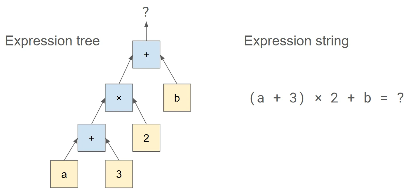
In data processing, expressions are often represented as a tree of operands and operators, where each leaf node is a column or a scalar, and each intersection is an operator (Figure 1). In the typical case, a scalar expression converts one or more inputs into a single output column. Scalar expressions typically represent a row-wise mapping between inputs and outputs, where each input row produces one output row.
For arithmetic expressions, there are three options for evaluation with cuDF: precompiled, AST (abstract syntax tree), and JIT transform.
The precompiled approach calls a libcudf public API for each operator in the expression, recursively computing the tree. Precompiled function calls in libcudf have the advantage of the broadest data type and operator support. The main disadvantage is that each operator materializes intermediates in GPU global memory during evaluation.
The AST approach uses the compute_column API in libcudf, which accepts the full tree as a parameter, and then uses a specialized kernel to traverse and evaluate the tree. AST execution uses a GPU thread-per-row parallelism model. The AST interpreter kernel is a useful tool for kernel fusion in cuDF, but it has limitations in its data type support and operator support.
The JIT transform approach in cuDF uses NVRTC to JIT compile a custom kernel for completing arbitrary transformations. NVRTC is a runtime compilation library for CUDA C++ that creates fused kernels at runtime. JIT compilation has the advantage of using optimized kernels for the expression to be evaluated. This means that the compiler is able to efficiently allocate GPU resources, rather than reserving GPU registers for the worst-case scenario.
As of cuDF 25.08, JIT transform adds support for several key operators that AST execution does not support, including ternary operator for if-else branching, and strings functions such as find and substring. The main disadvantage of JIT compilation is that the kernel compilation time of ~600 ms must either be paid at runtime or managed by prepopulating the JIT cache. This topic is addressed in more detail in subsequent sections of this post.
Using JIT transform
The rapidsai/cudf GitHub repo provides a suite of string_transforms examples to demonstrate string manipulation with both the precompiled approach and the new JIT transform approach. The example cases take the form of user-defined functions (UDFs) for string processing.
The example cases extract_email_jit JIT and extract_email_precompiled focus on a computation that takes an input string, confirms basic formatting of the string as an email address, and then extracts the email provider from the string. For a typical email address such as user@provider.com, the target output would be provider. In the case of malformed inputs, the example returns unknown as an alternate entry.
Figure 2 shows the extract_email_precompiled example, with logic highlighted in green identifying the “@” and “.” positions. Logic highlighted in pink computes an is_valid field based on the presence and location of “@” and “.” characters. Finally, logic highlighted in blue slices the provider from the input strings, and copies the alternate entry when the input is not valid. This approach yields correct results, but uses extra memory and compute to materialize the character positions, multiple Boolean columns, and the column containing the alternate entry.
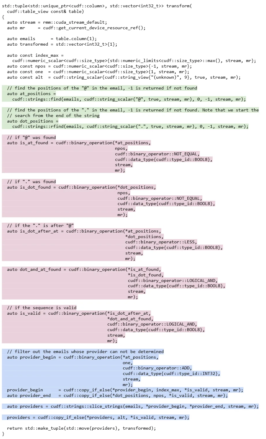
extract_email_precompiled highlighting the character detection logic (green), validation logic (pink), and result construction (blue)Using JIT compilation, you can create a GPU kernel that performs the same work more efficiently. Figure 3 shows the extract_email_jit example, which uses a raw string “udf” that defines the transformation. This process begins by finding and slicing at the “@” character, then finding and slicing at the “.” character.
The sequence of operations makes validation checking much simpler than processing the data as full columns in each step as in the precompiled example. The UDF uses standard C++ patterns like if-else branching and early returns to simplify the logic.
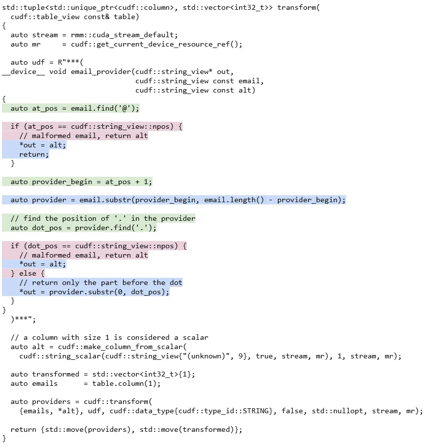
extract_email_jit highlighting the character detection logic (green), validation logic (pink), and result construction (blue)We encourage you to walk through the other examples to see more of these differences in action.
Performance benefits from JIT compilation
Using the JIT transform approach to process UDFs results in faster runtimes than using the precompiled approach. The primary source of speedup is due to the lower total kernel count in the JIT transform approach. When the same work can be performed with fewer kernels, the computations often have better cache locality and GPU registers can hold intermediates that would otherwise have to be stored in global memory for a subsequent kernel.
Figure 4 shows the timeline of kernel launches for the three string transformation examples, where blue bars represent kernels launched by the precompiled approach and green bars represent kernels launched by the JIT transform approach. The timeline data was collected with 200M input rows (12.5 GB input file size) on NVIDIA GH200 Grace Hopper Superchip hardware using a CUDA async memory resource. Note that kernels with <10 μs runtime have been omitted.
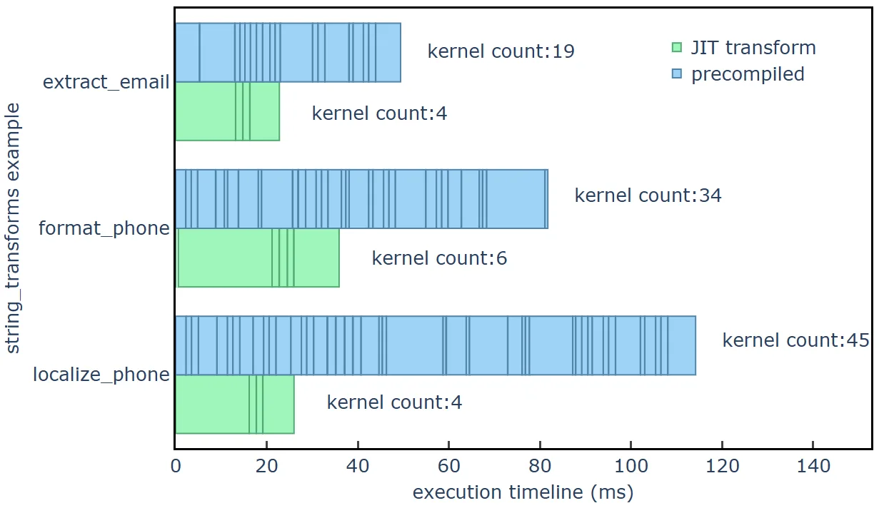
string_transformsThe JIT transform approach shows a benefit that scales with data size. At smaller data sizes, the JIT transform approach shows less overhead due to fewer kernel launches and this provides a speedup based on the complexity of the UDF. In addition to less overhead, the JIT transform approach uses less GPU memory bandwidth and compute resources which translates to even greater speedup versus the precompiled approach at larger data sizes.
Figure 5 shows speedups from 2x to 4x for the localize_phone example case and speedups from 1x to 2x for the simpler extract_email and format_phone example cases. Please note that the JIT transform approach processes about 30% larger data size before reaching the ~100 GB GPU memory limit on the Grace Hopper Superchip, due to fewer materialized intermediates.

string_transforms, plotted for file sizes 60 MB to 40 GBSpecial costs of JIT compilation
JIT compilation also brings some unique challenges to efficient execution. When the JIT transform approach runs the first time, cuDF will check a kernel cache located at the path specified by the environment variable LIBCUDF_KERNEL_CACHE_PATH. The cached kernel sizes in this example are about 130 KB. If a cached kernel is not found, JIT compilation time in the string_transforms example takes about 600 ms per kernel. If the kernel is found, then loading it takes about 3 ms.
Once compiled and loaded, subsequent calls to the kernel in the same process do not carry additional overhead. Figure 6 shows the first-run timing where each repetition is a new process and repetition 1 begins with an empty kernel cache. JIT-compiled times show higher wall time on first execution due to JIT compilation with NVRTC, and subsequent wall times drop dramatically. The wall time is reported as “warmup time” in the example, and data size is 200M rows.

For the examples in string_transforms, if JIT-compilation must be deferred until runtime, then the breakeven data size is about 1-3B rows processed in batches of ~100M rows. If the application layer pre-populates the JIT cache with previously compiled kernels, then JIT transforms typically yield benefits even from the first million rows.
Get started with efficient transforms in cuDF
NVIDIA cuDF provides powerful, flexible, and accelerated tools for working with expressions and UDFs. For more information about CUDA-accelerated dataframes, see the cuDF documentation and the rapidsai/cudf GitHub repo. For easier testing and deployment, RAPIDS Docker containers are also available for releases and nightly builds.
To get started with libcudf, the C++ submodule of cuDF, we recommend installing prebuilt binaries using the rapidsai-nightly Conda channel. Find the libcudf-example Conda package and install the string_transforms examples featured in this post. The libcudf-tests Conda package includes both unit tests and microbenchmarks so make it easy to run and profile cuDF precompiled and JIT compiled expression evaluators.