
This is the first post in a series about distilling BERT with multimetric Bayesian optimization. Part 2 discusses the set up for the Bayesian experiment, and Part 3 discusses the results.
You’ve all heard of BERT: Ernie’s partner in crime. Just kidding! I mean the natural language processing (NLP) architecture developed by Google in 2018. That’s much less exciting, I know. However, much like the beloved Sesame Street character who helps children learn the alphabet, BERT helps models learn language. Based on Vaswani et al’s Transformer architecture, BERT leverages Transformer blocks to create a malleable architecture suitable for transfer learning.
Before BERT, each core NLP task (language generation, language understanding, neural machine translation, entity recognition, and so on) had its own architecture and corpora for training a high performing model. With the introduction of BERT, there was suddenly a strong performing, generalizable model that could be transferred to a variety of tasks. Essentially, BERT allows a variety of problems to share off-the-shelf pretrained models and moves NLP closer to standardization, like how ResNet changed computer vision. For more information, see Why are Transformers important?, Sebastian Ruder’s excellent presentation Transfer Learning in Open-Source Natural Language Processing, or BERT: Pre-training of Deep Bidirectional Transformers for Language Understanding (PDF).
But BERT is really, really large. The BERT-Base is 110M parameters and BERT-Large is 340M parameters, compared to the original ELMo model that is ~94M parameters. This makes BERT costly to train, too complex for many production systems, and too large for federated learning and edge-computing.
To address this challenge, many teams have compressed BERT to make the size manageable, including HuggingFace’s DistilBert, Rasa’s pruning technique for BERT, Utterwork’s fast-bert, and many more. These works focus on compressing the size of BERT for language understanding while retaining model performance.
However, these approaches are limited in two ways. First, they do not tell you how well compression would perform on more application-focused methods, niche datasets, and directly on non-language understanding NLP tasks. Second, they are designed in a way that limits your ability to gather practical insights on the overall trade-offs between model performance and model architecture decisions. At SigOpt, we chose this experiment to begin to address these two limitations and give NLP researchers additional insight on how to apply BERT to meet their practical needs.
Inspired by these works, and specifically DistilBERT, we explored this problem by distilling BERT for question answering. Specifically, we paired distillation with multimetric Bayesian optimization. By concurrently tuning metrics like model accuracy and number of model parameters, you can distill BERT and assess the trade-offs between model size and performance. This experiment is designed to address two questions:
- By combining distillation and multimetric Bayesian optimization, can you better understand the effects of compression and architecture decisions on model performance? Do these architectural decisions (including model size) or distillation properties dominate the trade-offs?
- Can you leverage these trade-offs to find models that lend themselves well to application specific systems (productionalization, edge computing, and so on)?
Experiment design: data
Brought to you by the creators of SQUAD 1.1, SQUAD 2.0 is the current benchmark dataset for question answering. This classic question-answering dataset is composed of passages and their respective question/answer pairs, where each answer can be found as a sentence fragment of the larger context. By including unanswerable questions in the dataset, SQUAD 2.0 introduces an additional layer of complexity not seen in SQUAD 1.1. Think of this as your standard reading comprehension exam (without multiple choice), where you’re given a long passage and a list of questions to answer from the passage. For more information, see Know What You Don’t Know: Unanswerable Questions for SQuAD.
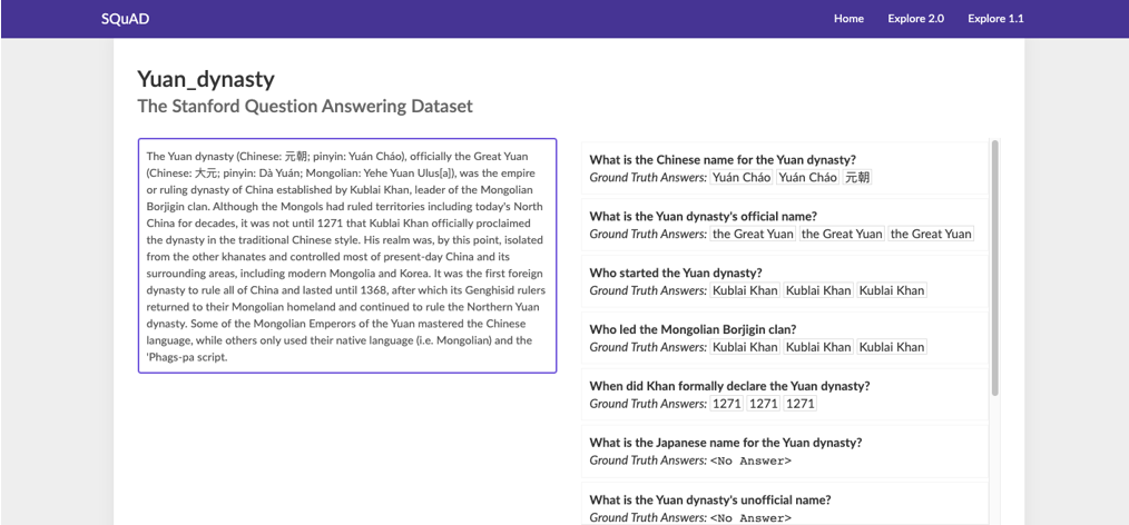
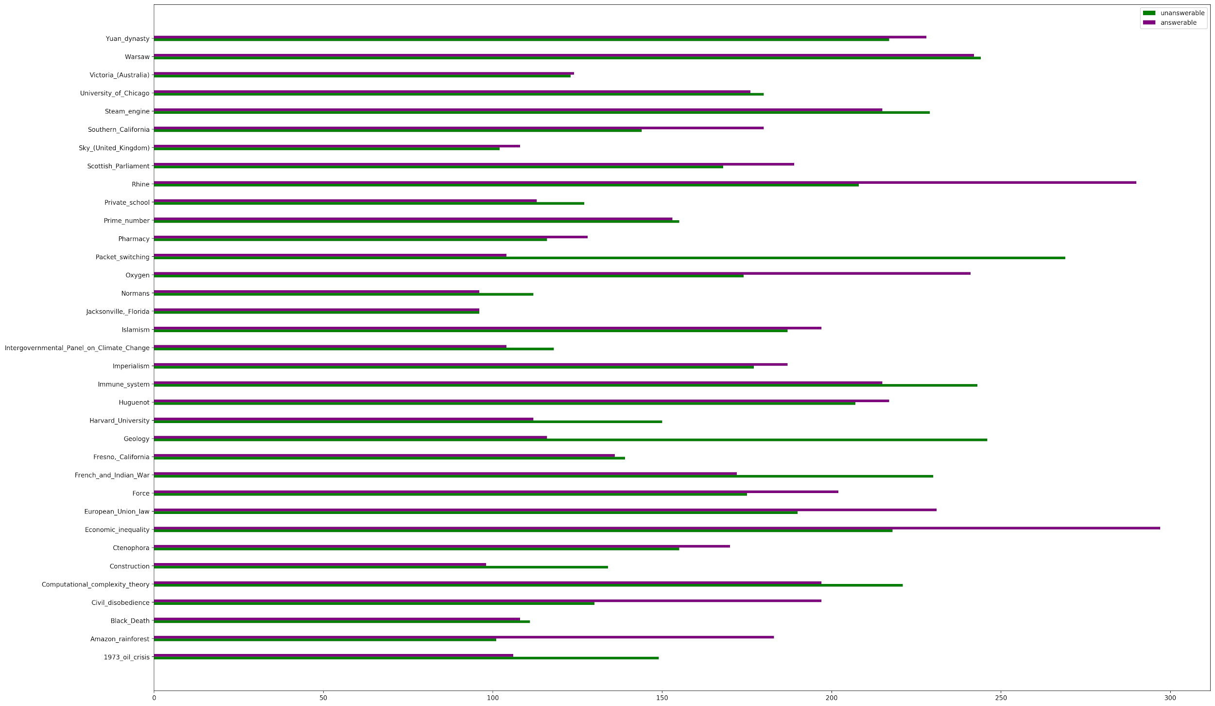
SQUAD 2.0 is split into 35 wide-ranging and unique topics, including niche physics concepts, a historical analysis of Warsaw, and the chemical properties of oxygen. Its broad range of topics make it a good benchmark dataset to access general question-answering capabilities.
Along with the 35 topics, the dataset is 50.07% unanswerable and 49.93% answerable. Answerable questions require the model to find specific strings within the context, but the unanswerable questions do not and only require the question to be classified as unanswerable.
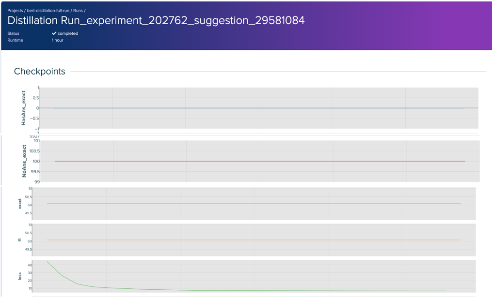
Although the addition of unanswerable questions makes the dataset more realistic, it forces the dataset to be unnaturally stratified. Essentially, a model could guess that all the questions are unanswerable and be 50% accurate. This is clearly not ideal, and you deal with this in an optimization setting later.
Experiment design: model
In this post series, you use the BERT architecture and HuggingFace’s Transformer package and model zoo for the implementation and pretrained models. You would not be able to conduct this experiment without these resources.
Distillation
To compress the model, use distillation and work with HuggingFace’s Distillation package and DistilBERT. Before looking into DistilBERT, here’s how distillation generally works.

The main idea behind distillation is to produce a smaller model (student model) that retains the performance of a larger model trained on the dataset (teacher model). Prior to the distillation process, the student model’s architecture (a smaller version of the teacher model) is chosen. For example, the teacher model is ResNet-150 and the student model is ResNet-13. For more information, see Distilling the Knowledge in a Neural Network.
During the distillation process, the student model is trained on the same dataset (or subset of the dataset) as the teacher model. The student model’s loss function is a weighted average of a soft target, dictated by the teacher’s output softmax layer, and a hard target loss, dictated by the true labels in the dataset (your typical loss function). By including the soft target loss, the student leverages the teacher model’s learned probabilistic distributions across classes. The student uses this information to generalize the same way as the teacher model and reach higher model performance than if it were to be trained from scratch. For more information, see the original paper, Distilling the Knowledge in a Neural Network, or Ujjay Upadhyay’s post, Knowledge Distillation.
Now that you understand distillation, here’s how distillation works for DistilBERT.
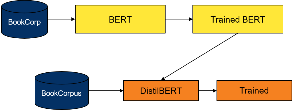
Both DistilBERT and BERT are trained on the BookCorpus and English Wikipedia (great corpuses for general language understanding). As with the general distillation process, the student model’s soft target loss comes from a pretrained BERT model’s output softmax layer, and the hard target loss comes from training the student model on the dataset. For more information, see Attention is All You Need (PDF) and DistilBERT, a distilled version of BERT: smaller, faster, cheaper and lighter (PDF).
In the next post, I set up the experiment design for searching for a student architecture and understanding the trade-offs between model size and performance during distillation. This includes how you search for student architecture, set up the distillation process, choose the right NVIDIA GPU, and manage orchestration.
Resources
- To re-create or repurpose this work, fork the sigopt-examples/bert-distillation-multimetric GitHub repo.
- For the model checkpoints from the results table, download sigopt-bert-distillation-frontier-model-checkpoints.zip.
- Download the AMI used to run this code.
- To play around with the SigOpt dashboard and analyze results for yourself, take a look at the experiment.
- To learn more about the experiment, view the webinar, Efficient BERT: Find your optimal model with Multimetric Bayesian Optimization.
- To see why methodology matters, see Why is Experiment Management Important for NLP?
- To use SigOpt, sign up for our free beta to get started.
- Follow the SigOpt Research & Company Blog to stay up-to-date.
- SigOpt is a member of NVIDIA Inception, a program that supports AI startups with training and technology.
Acknowledgements
Thanks to Adesoji Adeshina, Austin Doupnik, Scott Clark, Nick Payton, Nicki Vance, and Michael McCourt for their thoughts and input.
