
This is the third post in this series about distilling BERT with multimetric Bayesian optimization. Part 1 discusses the background for the experiment and Part 2 discusses the setup for the Bayesian optimization.
In my previous posts, I discussed the importance of BERT for transfer learning in NLP, and established the foundations of this experiment’s design. In this post, I discuss the model performance and model size results from the experiment.
As a recap of the experiment design, I paired distillation with multimetric Bayesian optimization to distill BERT for question answering and assess the trade-offs between model size and performance. What I found is that you can compress the baseline architecture by 22% without losing model performance, and you can boost model performance by 3.5% with minimal increase in model size. That’s is pretty great!
The rest of this post digs deeper into the results and answers the following questions:
- By combining distillation and multimetric Bayesian optimization, can you better understand the effects of compression and architecture decisions on model performance? Do these architectural decisions (including model size) or distillation properties dominate the trade-offs?
- Can you leverage these trade-offs to find models that lend themselves well to application specific systems (productionalization, edge computing, and so on)?
Multimetric optimization results
By using SigOpt’s multimetric optimization to tune the distillation process and model parameters, you can effectively understand the effects of compression and architecture changes on model performance.
Look at the results from the multimetric optimization experiment.
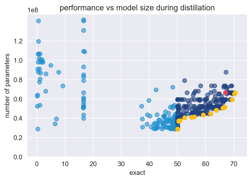
Each dot is an optimization run, or one distillation cycle. The yellow dots each represent a Pareto-optimal, hyperparameter configuration relative to the others. The pink dot is the baseline described earlier. The pale blue dots represent student models’ exact score that fell below the 50% metric threshold set for the experiment.
As I hoped, the multimetric experiment produces 24 sets of optimal model configurations depicted by the yellow dots in Figure 1. These sets of optimal configurations strongly fill out the Pareto frontier. Each point on the frontier provides a best possible trade-off between number of parameters and exact score. Due to the metric threshold set, the optimizer efficiently learns to avoid configurations that have models with less than 50% exact scores and focus on exploring configurations that perform well. In fact, 80% of the configurations suggested by SigOpt were either smaller or more accurate than the baseline. Seven model configurations were both smaller and higher performing than the baseline.
As the baseline (67.07% exact and 66.3 M parameters) is not on this frontier, this indicates that the model’s baseline configurations can still be pushed to reach an optimal trade-off point. The optimizer was able to find model architectures that are significantly smaller, with 96% of the frontier smaller than the baseline. The optimizer finds a significant number of configurations that are at or better performing than the baseline.
|
Scenario |
Frontier point: size |
Frontier point: exact score |
Size diff from baseline |
Exact score diff from baseline |
Link to Run |
|
Baseline |
66.3 M |
67.07% |
– |
– | |
|
Retain model size and maximize performance |
66.36M |
70.55% |
+0.09% params |
+3.45% | |
|
Minimize model size and maximize performance |
65.18M |
70.26% |
-1.69% params |
+3.19% | |
|
Minimize model size and retain performance |
51.40M |
66.82% |
-22.47% params |
-0.25% |
As Table 1 shows, you can increase the performance of the baseline model by ~3.50% with only a 0.09% increase in model size. On the flip side, you can shrink the model by ~22.50% parameters with only a 0.25% dip in model performance!
Most importantly, optimization results result in a large set of strong performing model configurations that you can choose from for your needs (instead of relying on a single architecture).
Looking at the parameter space
Now that you understand the trade-offs between model size and performance, look at which parameters heavily influence these trade-offs for each metric that was jointly optimized.
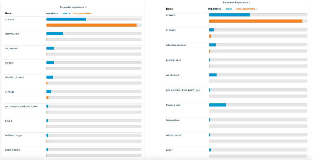
Unsurprisingly, both exact score and number of parameters are mainly influenced by the number of layers in the network. From the architecture search, you can see that the architectural parameters (num layers, num attention heads, and attention dropout) heavily influence the number of parameters, but a broader range of hyperparameters affect the exact score. Specifically, apart from num layers, exact score is dominated by the learning rate and three dropouts. In future work, it would be interesting to dig deeper to understand why the dropouts direct the model’s performance.
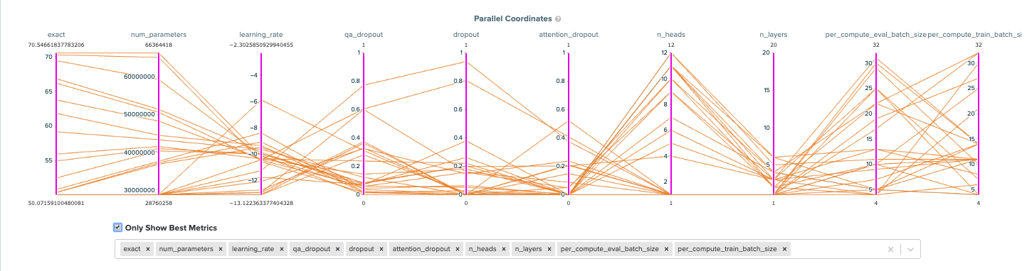
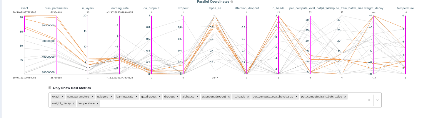
Looking at the parallel coordinates graphs and parameter importance charts, you can see that the model has a strong preference for the values of the number of layers, learning rate, and the three dropouts. When you look at the points on the frontier that perform at least as well as the baseline, stronger patterns emerge. Most interestingly, these high performing models weigh the soft target distillation loss (alpha_ce) much higher (at ~0.80) than the hard target distillation loss (at ~0.20). For architecture, the optimal values for all dropouts is close to 0.0, the number of layers center around 5, the number of heads center around 11, and specific attention heads are pruned given the size.
Model architecture and convergence
Now that you understand the hyperparameter space and parameter preferences, see if the optimized models converge and learn well. Using SigOpt’s dashboard, analyze the best performing models and smallest models (rows 2 and 4 in Table 1) architectures and training runs.
Best-performing model
Figure 5 shows that the best performing model retains both the number of layers and number of attention heads from the baseline. Unlike the baseline, it drops all the dropouts to 0, uses a significant number of steps to warm up, and heavily weighs the soft target loss.
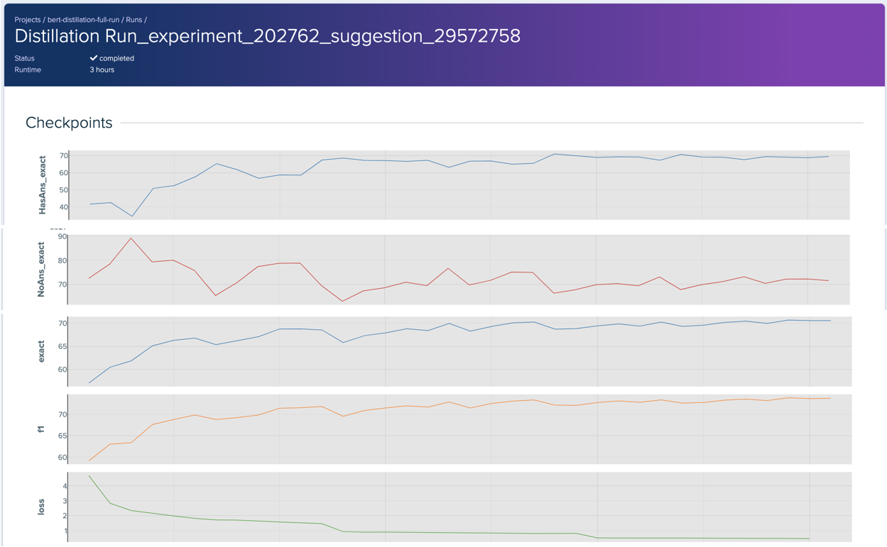
|
Parameter |
Value |
|
Weight for Soft Targets |
0.85 |
|
Weight for Hard Targets |
0.15 |
|
Attention dropout |
0 |
|
Dropout |
0.06 |
|
Learning Rate |
3.8e-5 |
|
Number of MultiAttention Heads |
12 |
|
Number of layers |
6 |
|
Pruning Seed |
42 |
|
QA Dropout |
0.04 |
|
Temperature |
3 |
|
Warm up steps |
52 |
Smallest model
The smallest model uses four layers of Transformer blocks and prunes a single attention head from each one. Much like the best performing model, it also weighs the soft target loss over the hard target loss and uses no dropout. Interestingly, it uses the highest possible number of warm up steps in its learning strategy.
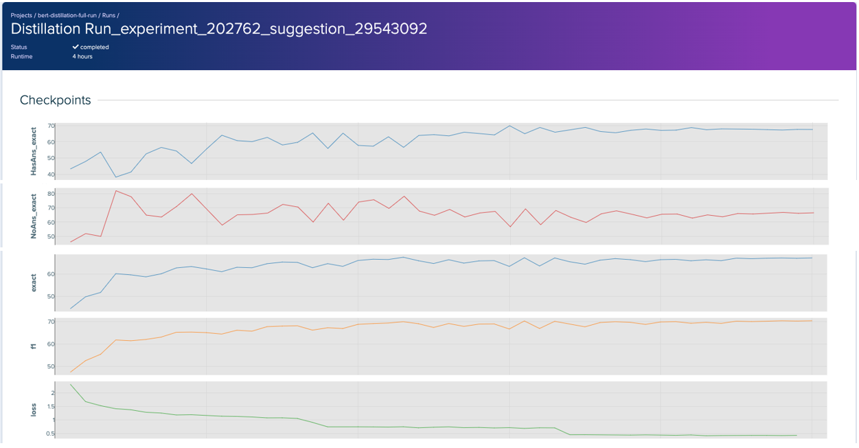
|
Parameter |
Value |
|
Weight for Soft Targets |
0.83 |
|
Weight for Hard Targets |
0.17 |
|
Attention dropout |
0 |
|
Dropout |
0.05 |
|
Learning Rate |
5e-5 |
|
Number of MultiAttention Heads |
11 |
|
Number of layers |
4 |
|
Pruning Seed |
92 |
|
QA Dropout |
0.06 |
|
Temperature |
5 |
|
Warm up steps |
100 |
Much like the baseline, both models converge and aptly learn the distinction between answerable and unanswerable questions. Both models seem to learn similarly, as they have similar performance and loss curves. The main difference is in how they can correctly classify and answer answerable questions. While both models initially struggle and dip in performance for “HaAns_exact”, the larger model can quickly learn and start recognizing answerable questions. The smaller model begins to climb out of the dip but quickly stagnates in its ability to recognize answerable questions. The best performing model might be able to learn these more complex patterns as it is a larger model in terms of the number of layers and attention heads.
By using SigOpt’s multimetric optimization to tune the distillation process, you can understand the trade-offs between model size and performance, get insights on your hyperparameter space, and validate the training runs. Beyond understanding your trade-offs, you can make informed decisions for your model architecture, hyperparameters, and distillation process that suit your own modeling workflows and production systems. At the end of the process, you can identify different configurations that made optimal tradeoffs between size and accuracy, including seven that were better in both metrics as compared to the baseline.
Analyzing the best performing model
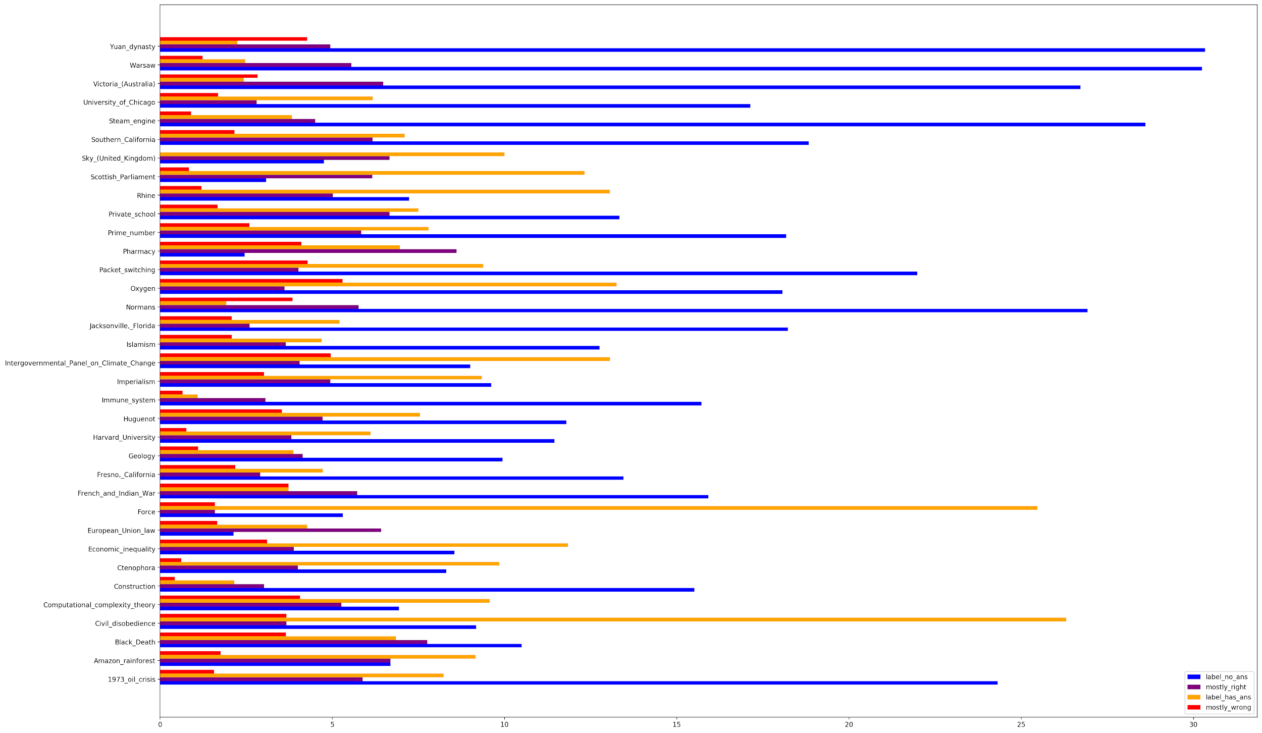
The best performing model (from the results earlier) achieves 70.55% on the exact score. Take a closer look to understand how well the model answers questions.
To evaluate the model performance, look at how accurately it classifies unanswerable questions, how accurately it answers answerable questions, and why it fails to do either. The model’s accurate classifications follow the Exact score guidelines and expects the exact string score to be the correct answer. The model’s misclassifications are split into four categories:
- Mostly correct: answer predictions that are almost the right string, give or take a punctuation or preposition.
- Mostly wrong: predictions that are unlike the true answer.
- Label has answer: predictions that claim questions are unanswerable when the questions are answerable.
- Label has no answer: Predictions that answer questions with no answers.
This stratification helps you understand where the model falters and how to improve model performance in future work.
Looking at the broader buckets of correct and incorrect predictions, the model overwhelmingly predicts the right answer for all the topics in SQUAD 2.0, with some topics such as the Yuan Dynasty, Warsaw, and Victoria, Australia having more incorrect answers than most.
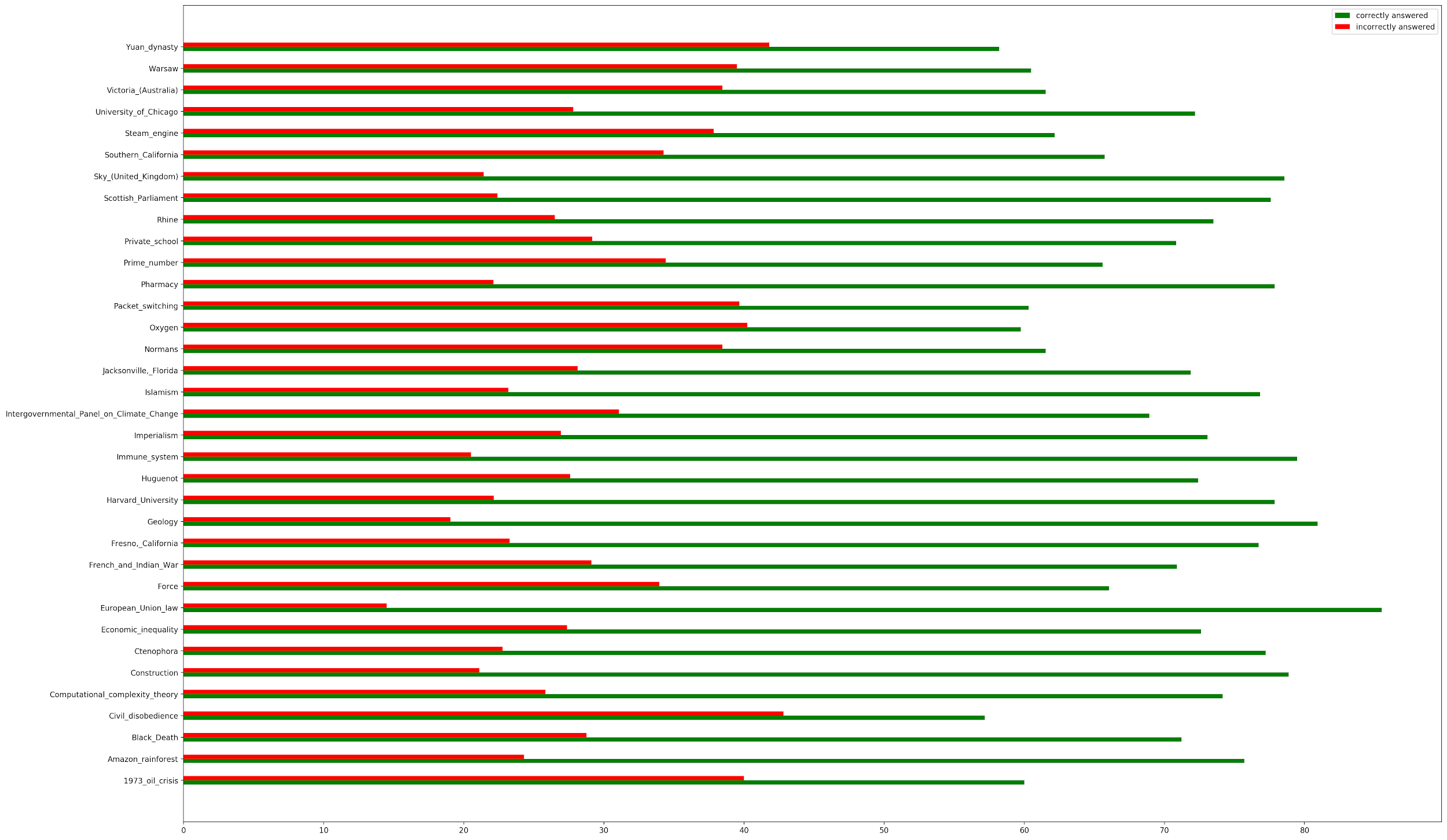
When you break the incorrect answers up into their four categories, most of the incorrect predictions are characterized by the model predicting answers for unanswerable questions. Furthermore, there is the least number of incorrect answers due to the model answering questions with completely wrong information. You continue to see topics such as the Yuan Dynasty, Warsaw, and the steam engine confusing the model.
Why does this matter?
Building small and strong performing models for NLP is hard. Although there is great work currently being done to develop such models, it is not always easy to understand how the decisions and trade-offs were made to arrive at these models. In this experiment, you leverage distillation to effectively compress BERT and multimetric Bayesian optimization paired with metric management to intelligently find the right architecture and hyperparameters for a compressed model. By combining these two methods, you can more thoroughly understand the effects of distillation and architecture decisions on the compressed model’s performance.
You can gain intuition on your hyperparameter and architectural parameter space, which helps you make informed decisions in future, related work. From the Pareto frontier, you can practically assess the trade-offs between model size and performance and choose a compressed model architecture that best fits your needs.
Resources
- To re-create or repurpose this work, fork the sigopt-examples/bert-distillation-multimetric GitHub repo.
- For the model checkpoints from the results table, download sigopt-bert-distillation-frontier-model-checkpoints.zip.
- Download the AMI used to run this code.
- To play around with the SigOpt dashboard and analyze results for yourself, take a look at the experiment.
- To learn more about the experiment, view the webinar, Efficient BERT: Find your optimal model with Multimetric Bayesian Optimization.
- To see why methodology matters, see Why is Experiment Management Important for NLP?
- To use SigOpt, sign up for our free beta to get started.
- Follow the SigOpt Research & Company Blog to stay up-to-date.
- SigOpt is a member of NVIDIA Inception, a program that supports AI startups with training and technology.
Acknowledgements
Thanks to Adesoji Adeshina, Austin Doupnik, Scott Clark, Nick Payton, Nicki Vance, and Michael McCourt for their thoughts and input.
