
This post is the second in a series on Autonomous Driving at Scale, developed with Tata Consultancy Services (TCS). The previous post in this series provided a general overview of the deep learning inference for object detection. In this post, we dive deep into the object detection inference process. We cover an explanation of the object detection metrics and how to interpret them with empirical data. The next post discusses optimization techniques and deployment of an end-to-end inference pipeline.
All the code for the YOLOv3-based object detection inference process is available in the eriklindernoren/PyTorch-YOLOv3 GitHub repo.
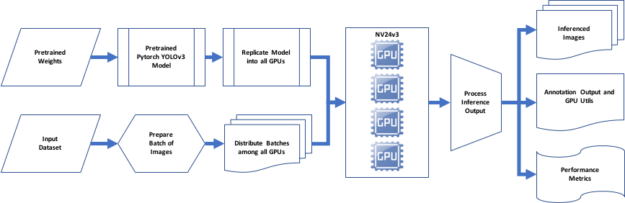
To review, we used the full version YOLO configuration file. It contains information about the network, convolution layers, three YOLO detection layers, and other layers along with their properties. We used PyTorch to parse the configuration file and apply the model definition to implement the network. The YOLOv3 detection layers have CUDA enabled by default. PyTorch CUDA, from the NGC software hub offering GPU optimized containers, is preconfigured with libraries like cuDNN to leverage multiple CUDA-capable processors.
Next, we loaded the pretrained bias and weights file for YOLOv3-416, which connects the nodes between the layers. The convolution layers use the learnable parameters, that includes the weights of the kernel and the bias. The weights are specified as 3D tensor, with number of rows, columns, and channels. We used zero-padding throughout the network to maintain the dimension of the images. The input layer contains no learnable parameters as it includes the data. Also, the shortcut and routing layers have no weights as they do not perform any convolutions.
The number of learnable parameters for the convolution layers is determined by the following formulas:
weights + biases
inputs x outputs + biases
If the last layer is dense, then inputs = # of nodes
If the last layer is conv, then inputs = # of filters
outputs = (# of filters) x (size of filters)
biases  = # of filters
The number of learnable parameters for the output layer is determined by the following formulas:
weights + biases
inputs x outputs + biases
inputs = image width x image height x # of filters
Because it is a dense layer, outputs = # of nodes
biases  = # of nodes
The network downsamples the image by a factor called the stride of the kernel of a convolutional layer of the network. With an input of 416 x 416, detections are performed on scales of 13 x 13 with stride 32, 26 x 26 with stride 16, and 52 x 52 with stride 8. At every scale, each cell predicts three bounding boxes using three anchors (different at different scales), for a total of nine anchors.
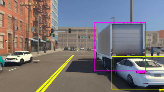
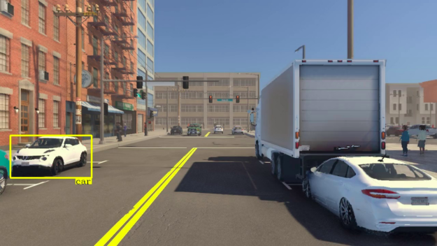
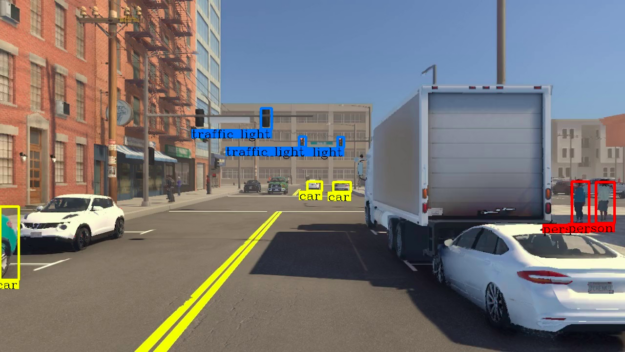
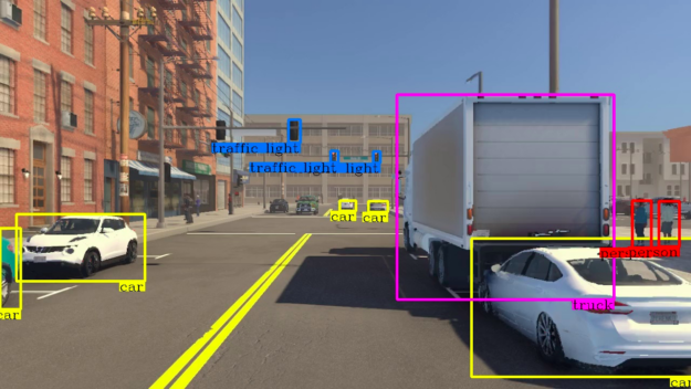
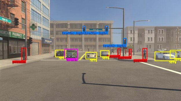
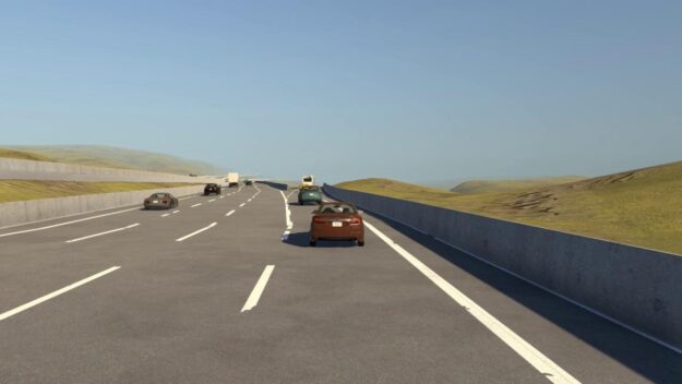
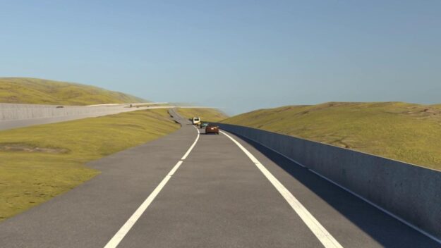
Weights based on predicted probabilities are associated with the bounding boxes—subsequently, we threshold the detections by some value to only see high scoring detections. Finally, non-maximum suppression (NMS) is used to remove multiple detections to select one bounding box per detected object to generate the consolidated inference image output.
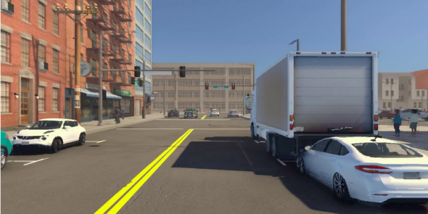
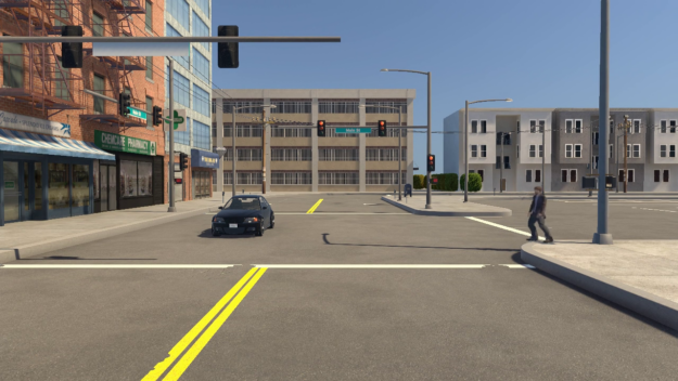
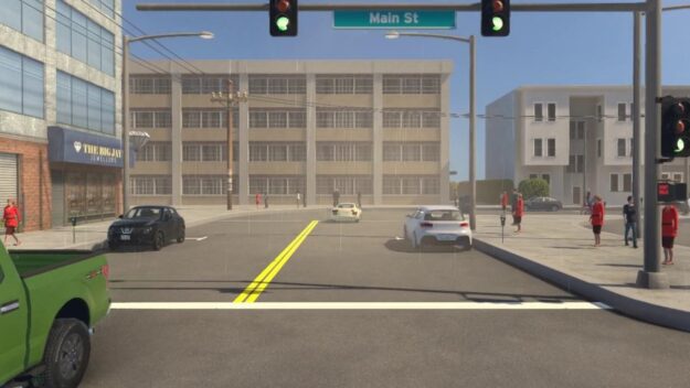
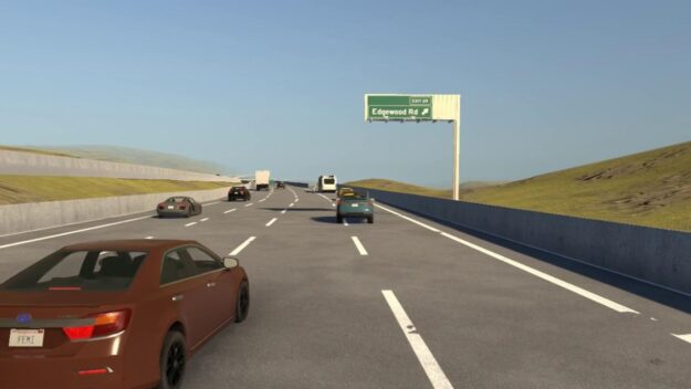
Inference output
Inference performance metrics
The object detection inference process is responsible for performing image classification and localization. Each image can have multiple objects of different categories for classification and localization. The object categories detected include car, truck, bus, pedestrian, and traffic light. The object detection performance metrics serve as a measure to quantifiably assess how well the inference performs on image classification, localization, and object detection tasks.
Evaluating image classification
Classifying images is a hard problem, and accurate classification is even harder. For pre-annotation, we seek to balance speed and image classification accuracy. The terms image and object are used interchangeably in this section.
The task in image classification is to predict a single label (or a distribution over labels with confidence) for a given image. Images are 3D arrays of integers from 0 to 255, of size width x height x 3. The three represents the color channels: red, green, and blue.
The following are the known list of challenges when classifying an image that affects the image inference speed and accuracy. We encountered these with our dataset. Also, mentioned are the techniques and tricks where applicable that are incorporated in YOLOv3 to address these challenges. It is important to note that a significant number of contributions came from many prior research efforts. Classification with Deep Convolutional Networks is probably one of the most influential research papers, among other notable research works:
- 2014 – Very Deep Convolutional Neural Networks for Large-Scale Image Recognition
- 2015 – Going Deeper with Convolutions
- 2015 – Deep Residual Learning for Image Recognition
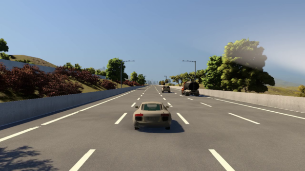
Viewpoint variation
The object’s orientation can vary depending on the camera sensor position.

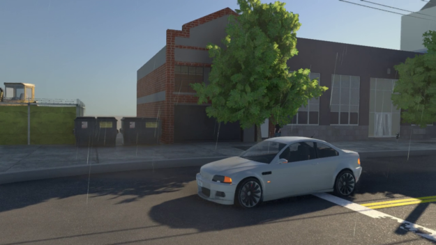
YOLOv3 false positives per image (FPPI) varies with the viewpoint. It depends on the camera-sensor positioning and the impact of the field of view (FOV). In some instances, larger FFPI is attributed to images captured from the single front camera.
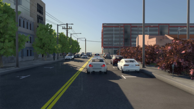
Scale variation
The objects often exhibit variation in their size (size in the real world, not only in terms of their extent in the image).
YOLOv3 makes predictions at three scales, from detecting large objects to small objects, although it is not robust in detecting far-away smaller objects.
Distortion
Many objects of interest are not rigid bodies. In extreme cases, they can be deformed in extreme ways.
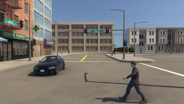
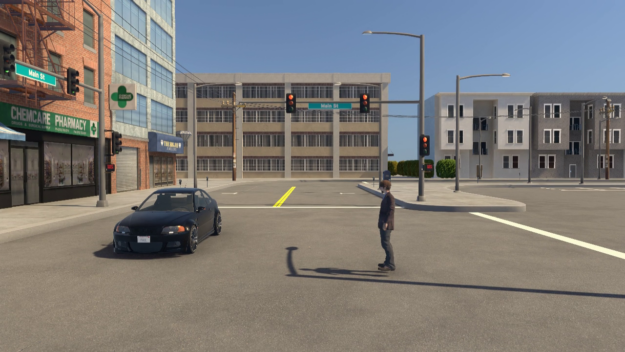
YOLOv3 is more accurate in predicting cars, trucks, buses, and traffic lights because they are rigid objects with a well-known geometry. However, as pedestrians are not rigid bodies and have various poses and deformations, there are better network structures to make more accurate pedestrian detection.
Occlusion
The objects of interest can be occluded. Sometimes only a small portion of an object (as little as few pixels) could be visible.

CNN-based object detection methods like YOLOv3 have a disadvantage, requiring feature map generation to be robust against object occlusion. Also, merely raising many feature maps does not improve performance. Methods like spatial pyramid pooling are known to better handle occlusion by improving the conventional YOLOv3 algorithm.
Illumination conditions
The effects of illumination are drastic on the pixel level.
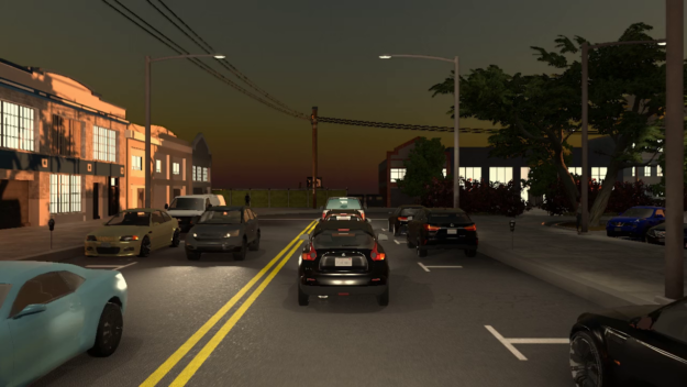
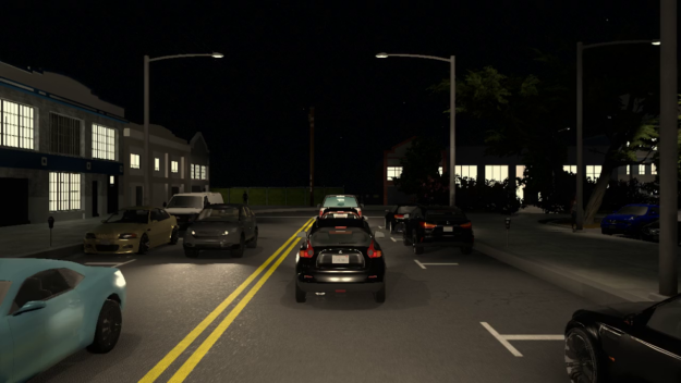
Results show that YOLOv3 classification and localization are affected by illumination uniformity.
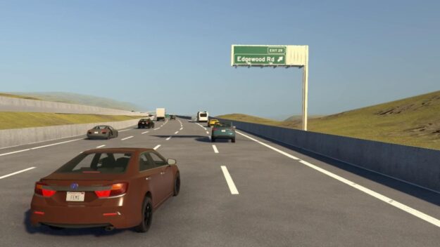
Background
The objects of interest may blend into their environment, making them hard to identify.

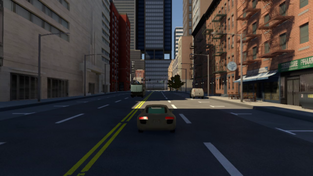
YOLOv3 traverses the entire input image in predicting boundaries. With the additional context, YOLO demonstrates fewer false positives in background areas.
Inter-class variability
The classes of interest can often be relatively broad, such as vehicles. There are many different types of vehicles, each with their own appearance.
YOLOv3 maximizes the inter-class variability by refraining from softmaxing the classes. Instead, the prediction of each class score uses logistic regression with a threshold.
Intra-class variability
Objects of the same class can look vastly different.


YOLOv3 performs object recognition well, irrespective of the intra-class variability present in the image frames. Accuracy is the proportion of correct results among the total number of cases examined.
Classification accuracy = How many were predicted/Actual number of ground-truth labels
| Class | Ground-truth label count |
| Cars | 1,078,642 |
| Bus | 33,307 |
| Truck | 63,128 |
| Pedestrian | 62,837 |
| Traffic Light | 827,182 |
| Total label count (all classes combined) | 2,065,096 |

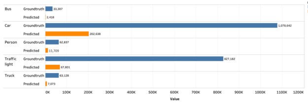
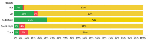
| Class | Correct predictions (Count) | Overall accuracy (%) | Accuracy by class (%) |
| Car | 172,583 | 8 | 16 |
| Truck | 2,525 | 1 | 4 |
| Bus | 2,332 | 1 | 7 |
| Traffic Light | 33,087 | 2 | 4 |
| Pedestrian | 15,709 | 7 | 25 |
As observed, the classes are not well balanced from an accuracy perspective, thus they are not a suitable choice for the model’s image classification performance in autonomous vehicle development.
The object detection accuracy falls short of identifying correct predictions from the overall predictions.
The overall low accuracy also seems to indicate that the MSCOCO dataset used as training data for YOLOv3 model-building is not strictly representative of the input dataset. This dataset shift has resulted in significant underperformance. The training dataset selection bias and dynamic ambient conditions that are prevalent in the autonomous vehicle context is a pervasive problem that needs addressing to improve object detection accuracy.
The low object detection accuracy can be improved by retraining using transfer learning from the pretrained YOLOv3 model. In the training stage, the CNN framework initializes the pretrained YOLOv3 model. Fine-tuning various layers of the network using the custom dataset yields better object detection accuracy.
The pretrained YOLOv3 model retraining process is a topic for another post. However, for this post, we further evaluated performance metrics culminating in mAP. The performance metrics are measured, keeping all the configurable parameters unaltered, including Intersection Over Union (IOU) threshold, the objectiveness confidence, and NMS threshold so that you can compare the model performance with the benchmark MSCOCO dataset. The objective of the pretraining process is to close the performance gap.
While accuracy measures the fraction of correct predictions, precision measures the fraction of actual positives among all predicted positives and recall measures the number of real positives predicted as positives.
For each class, use the following formula:
Precision = How many of the predicted are positive/Total predicted
Recall = How many of the predicted are positive/Actual number of ground-truth labels
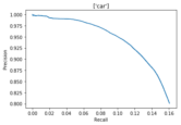
The precision and recall curve is an excellent way to evaluate the performance of an object detector as the confidence is changed by plotting a graph for each object class.
- An object detector of a class is good if its precision stays high as recall increases, by varifying the confidence threshold, the precision and recall are still high.
- A weak object detector that needs to increase the number of detected objects ( lower precision) to retrieve all ground-truth objects (high recall), starting with high precision values and decreasing as recall increases.
Other characteristics of a sound object detector include:
- A high precision (0 false positives) detector that can identify only relevant objects
- A high recall (0 false negatives) detector that can find all ground truth
A single-number evaluation metric, called the F1 score, helps control the tradeoff between precision and recall.
F1 score = 2*Precision*Recall/(Precision + Recall)
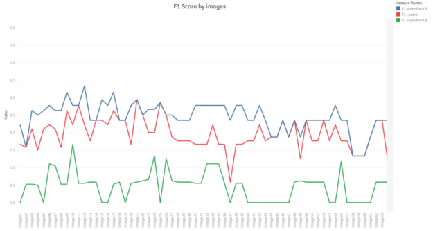
When both precision and recall are high, the F1 score is high. For all other results, the F1 score is low.
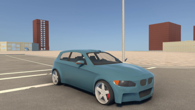
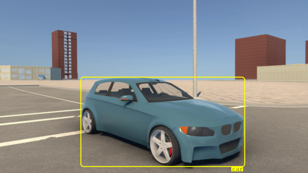
Evaluating object localization
The object detection process requires the object to be localized as well. We used IOU to compare the predicted bounding box with the ground-truth bounding box.
IOU = intersection area of the two predicted bounding box and corresponding ground-truth bounding box/intersection area of the two predicted bounding box and corresponding ground-truth bounding box
The range of the IOU can be described as 0 <= IOU <= 1, where zero indicates no overlap, and IOU shows a perfect overlap. Typically, boxes with a certain IOU threshold determine the candidate predicted bounding boxes. We used a 0.5 IOU threshold, the same as the benchmark IOU threshold used by the YOLOv3 algorithm.
The NMS component added to the YOLOv3 object detection algorithm also uses the IOU concept to make the algorithm perform better. NMS calculates the IOUs to remove multiple detections to select one bounding box per detected object to generate the inference localized image output.
Evaluating object detection
It is helpful to have a single-number metric when determining the performance of the model given the input dataset.
Mean Average Precision (“mAP”) is the mean of the Average Precisions per class, as shown in the following table calculated at an IOU threshold of 0.5, the same as the benchmark IOU threshold used by the YOLOv3 algorithm.
| AP (Car) | 25 |
| AP (Bus) | 15 |
| AP (Truck) | 15 |
| AP (Traffic Light) | 25 |
| AP (Person) | 40 |
| mAP | 24 |
As the IOU threshold increases, mAP reduces. Given that YOLOv3 makes predictions at three scales, you could compute the mAP for small, medium, and large objects separately, and the performance can vary significantly from low to high, respectively.
Summary
Addressing sensitivities of variations in data distribution, data type, annotation requirements, quality parameters, the volume of data, and the effectiveness of automation is critical to achieving optimal annotation accuracy and speed.
The NVIDIA GPU-accelerated, PyTorch YOLOv3-based, object detection inference pipeline shows some of the typical challenges in real-world environment data affected, for example, by illumination, rotation, scale and occlusion when annotating autonomous data. This work serves as an outline for creating an optimized, end-to-end, scalable pipeline supported by inference performance metrics, which helps as a measure to assess the quality of the annotation inference output performed on the input dataset.
For more information about how to optimize and accelerate model training or inferencing and develop a configurable annotation pipeline, see Part 3 in this series, Optimization and Deployment.
Tata Consultancy Services (TCS) is an IT services, consulting and business solutions organization that has partnered with many of the world’s largest businesses in their transformation journeys for the last 50 years. TCS offers a consulting-led, cognitive- powered, integrated portfolio of IT, business and technology services, and engineering. This is delivered through its unique Location Independent Agile delivery model, recognized as a benchmark of excellence in software development. TCS has more than 448,000 employees in 46 countries with $22 billion in revenues as of March 31, 2020.
TCS Automotive Industry Group focuses on delivering solutions and services to address the CASE ( Connected, Autonomous, Shared and Electric) ecosystem and partners with industry-leading players to address the opportunities evolving from disruption in the automotive industry.
To stay up-to-date on TCS news in North America, follow us on Twitter @TCS_NA and LinkedIn @Tata Consultancy Services – North America. For TCS global news, follow @TCS_News.
