You’ve probably seen headlines about innovation in automated driving now that there are several cars available on the market that have some level of self-driving capability. I often get questions from colleagues on how automated driving systems perceive their environment and make “human-like” decisions.
The autonomous car in Figure 1 must locate and classify all the relevant objects on the road (in this case other vehicles) so that it can brake or safely maneuver around vehicles or pedestrians. The system also must detect lane markers in order to center the car within its lane. Deep learning enables machines to detect and classify objects of interest more accurately than people can and is becoming the primary enabling technology for environment perception.
In this post we’ll explain how deep learning is used to solve two common perception tasks for automated driving:
- Vehicle detection
- Lane detection
We’ll be using MATLAB’s new capabilities for deep learning and GPU acceleration to label ground truth, create new networks for detection and regression, and to evaluate the performance of a trained network.
Vehicle Detection
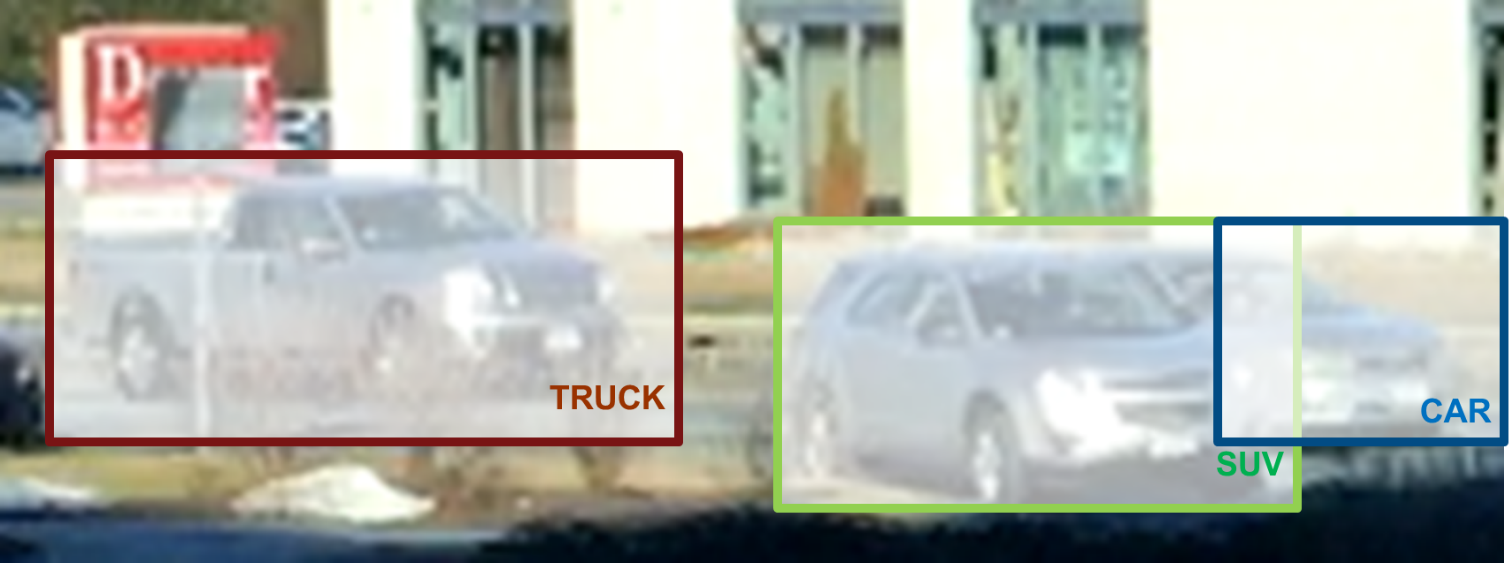
Object detection is used to locate pedestrians, traffic signs, and other vehicles. In this section we’ll use a vehicle detection example to walk you through how to use deep learning to create an object detector. The same steps can be used to create any object detector. Figure 2 shows the output of a three class vehicle detector, where the detector locates and classifies each type of vehicle.
Before we can start creating a vehicle detector, first we need a set of labeled training data, which is a corpus of images annotated with the locations and labels of objects of interest. More specifically, someone needs to sift through every image or frame of video and label the locations of all objects of interest. This process is known as ground truth labeling. Ground truth labeling is often the most time-consuming part of creating a vehicle detector. Figure 4 shows a raw training image on the left, and the same image with the labeled ground truth on the right.

As you can imagine, labeling a sufficiently large set of training images can be a laborious, manual process. To reduce the amount of time we spent labeling data, we used MATLAB Automated Driving System Toolbox, which provides an app to label ground truth as well as automate part of the labeling process. Figure 4 shows a screenshot of the Ground Truth Labeler app that we use to label training data.
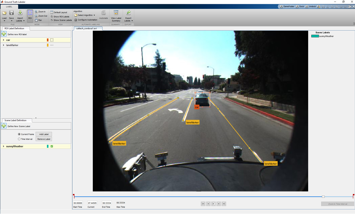
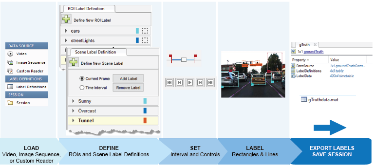
One way to automate part of the process is to use a tracker. The tracker we use is the Kanade Lucas Tomasi algorithm (KLT) which is one of the first computer vision algorithms to be used in real-world applications. The KLT algorithm represents objects as a set of feature points and tracks their movement from frame to frame. This lets us manually label one or more objects in the first frame, and use the tracker to label the rest of the video. The Ground Truth Labeler app also allows users to import their own algorithms to automate labeling. The most common way we’ve seen this feature used is when users import their own existing detectors to label new data, which helps them eventually create more accurate detectors. Figure 5 illustrates the workflow used to label a sequence of images or a video using the Ground Truth Labeler app.
The labeled data is stored as a table that lists the location of the vehicles in each time step of video from our training set. With the ground truth labelling complete, we can start training a vehicle detector. In our case we estimate we sped up the process of ground truth labeling by up to 119x. The training video data for our video was captured at 30 frames per second, and we labeled objects every 4 seconds. That means we saved the time it would take to label the 119 frames in between. This 119x savings is a best case as we sometimes had to correct the output of the automated labeling.
To train a vehicle detector, we use the new deep learning framework in MATLAB. To speed up the training process, we use an NVIDIA™ GPU (a Tesla K40c). This can speed up the training time by over 100x vs. CPU-only training. We highly recommend using a CUDA-capable NVIDIA GPU with compute capability 3.0 or higher. If you have access to multiple GPUs, it’s easy to use them with the same MATLAB code and a single setting change.
For our vehicle detector, we use a Faster R-CNN network. Let’s start by defining a network architecture as illustrated in the MATLAB code snippets below. The Faster R-CNN algorithm analyzes regions of an image and therefore the input layer is smaller than the expected size of an input image. In our case we choose a 32×32 pixel window. The input size is a balance between execution time and the amount of spatial detail you want the detector to resolve.
% Create image input layer.
inputLayer = imageInputLayer([32 32 3]);
The middle layers are the core building blocks of the network, with repeated sets of convolutional, ReLU and pooling layers. For our example, we’ll use just a couple of layers. You can always create a deeper network by repeating these layers to improve accuracy or if you want to incorporate more classes into the detector.
% Define the convolutional layer parameters.
filterSize = [3 3];
numFilters = 32;

% Create the middle layers.
middleLayers = [

    convolution2dLayer(filterSize, numFilters, 'Padding', 1)
    reluLayer()
    convolution2dLayer(filterSize, numFilters, 'Padding', 1)
    reluLayer()
    maxPooling2dLayer(3, 'Stride',2)

    ];
The final layers of a CNN are typically a set of fully connected layers and a softmax loss layer. In this case, we’ve added a ReLU nonlinearity between the fully connected layers to improve detector performance since our training set for this detector wasn’t as large as we would like.
finalLayers = [

    % Add a fully connected layer with 64 output neurons. The output size
    % of this layer will be an array with a length of 64.
    fullyConnectedLayer(64)

    % Add a ReLU non-linearity.
    reluLayer()

    % Add the last fully connected layer. At this point, the network must
    % produce outputs that can be used to measure whether the input image
    % belongs to one of the object classes or background. This measurement
    % is made using the subsequent loss layers.
    fullyConnectedLayer(width(vehicleDataset))

    % Add the softmax loss layer and classification layer.
    softmaxLayer()
    classificationLayer()
];

layers = [
    inputLayer
    middleLayers
    finalLayers
    ]
To train the object detector, we pass the layers network structure to the trainFasterRCNNObjectDetector function. If you have a GPU installed, the algorithm will default to using the GPU. If you want to train without a GPU (something that is not recommended) or use multiple GPUs, you can do so by adjusting the ExecutionEnvironment parameter in trainingOptions. In our tests, using an NVIDIA Titan X GPU was 30 times faster than using a CPU (Intel Xeon E5-2686v4) to train a Faster R-CNN vehicle detector. On average the CPU took a little over 600 seconds while training with a GPU took just 20 seconds.
detector = trainFasterRCNNObjectDetector(trainingData, layers, options, ...
        'NegativeOverlapRange', [0 0.3], ...
        'PositiveOverlapRange', [0.6 1], ...
        'BoxPyramidScale', 1.2);
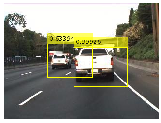
Once training is done, try it out on a few test images to see if the detector is working properly. We used the following code to test the detector on a single image. Figure 6 shows the output.
% Read a test image.
I = imread('highway.png');

% Run the detector.
[bboxes, scores] = detect(detector, I);

% Annotate detections in the image.
I = insertObjectAnnotation(I, 'rectangle', bboxes, scores);
figure
imshow(I)

Once you are confident that your detector is working, we highly recommend testing it on a larger set of validation images using a statistical metric such as average precision which provides a single score measure of the ability of the detector to make correct classifications (precision) and the ability of the detector to find all relevant objects (recall). This page provides more information on how you can evaluate a detector.
Lane Detection
Lane detection is the identification of the location and curvature of lane boundaries of visible lanes on a roadway. This is useful to help a vehicle center it’s driving path and safely navigate lane changes. Unlike the previous example where our algorithm had to predict the class of the vehicle (classification) as well as its location (bounding box), in this case we need the algorithm to output a set of numbers that represent the coefficients of parabolas that represent the right and left lane boundaries. To solve this, we will construct a CNN that performs regression to output the coefficients.
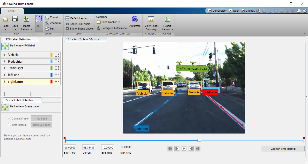
Similar to the previous example, the first step in the process is to label a set of training data with the ground truth representing the right and left lane boundaries. As in the previous section, we recommend using the Ground Truth Labeler app in MATLAB Automated Driving System Toolbox. Notice how we’ve labeled the lane boundaries using poly-lines in the figure below in addition to other objects that are labeled using rectangular bounding boxes.
To get a little insight on the ground truth for lane boundaries, Figure 8 shows the table we used to store the coefficients. Notice each column represents one of the coefficients of the parabola.

You’ll notice that we have just 1225 training samples for this task, which is usually not sufficient to train a deep network. The reason this is OK is that we will use transfer learning, by starting with a pre-existing network that was trained on a massive set of images and adapting it for the task. The network we’ll use as a starting point is AlexNet, trained to recognize 1000 different categories of images.
You can load a pre-trained AlexNet model into MATLAB with a single line of code. Note that MATLAB allows you to load other models like VGG-16 and VGG-19, or import models from the Caffe ModelZoo.
originalConvNet = alexnet
Once we have the network loaded into MATLAB we need to modify its structure slightly to change it from a classification network into a regression network. Notice in the code below that I have 6 outputs corresponding to the three coefficients for the parabola representing each lane boundary.
%Extract layers from the original network
layers = originalConvNet.Layers

%Net surgery
%Replace the last few fully connected layers with suitable size layers
layers(20:25) = [];
outputLayers =  [ ...
  fullyConnectedLayer(16, 'Name', 'fcLane1');
  reluLayer('Name','fcLane1Relu');
  fullyConnectedLayer(6, 'Name', 'fcLane2');
  regressionLayer('Name','output')];
layers = [layers; outputLayers]
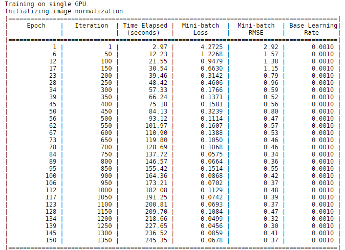
When we trained this network, we used an NVIDIA Titan X (Pascal) GPU. As you can see in Figure 9, it took 245 seconds to train the network. This time is lower than we expected mostly due to the fact that only a limited number of weights from the new layers are being learned, and also because MATLAB automatically uses CUDA and cuDNN to accelerate the training process when a GPU is available. In our tests using a GPU was over 100 times faster to train the lane boundary detection network than using a CPU. The 100x speedup using a GPU was computed over 1000 iterations. We did not fully time how long it took to train the entire network on a CPU, but we extrapolated that it would take over 6 hours.
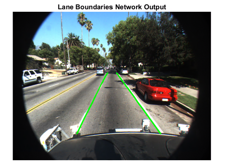
Despite the limited number of training samples, the network performs extremely well and is able to accurately detect lane boundaries, as Figure 10 shows.
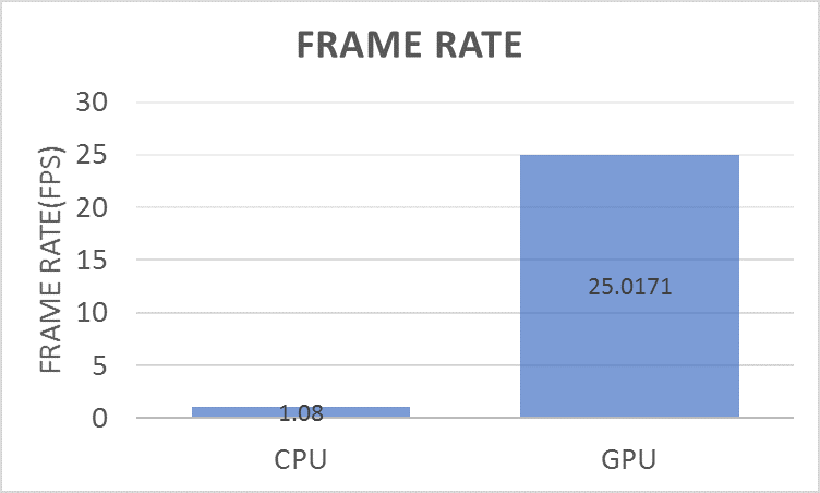
We also benchmarked the inference performance improvement on a GPU compared to a CPU. To estimate the frame rate, we timed how long it took for the lane boundary detection network to process 250 frames of video. Figure 11 shows the performance of the CPU and GPU on this task. Notice that it is ~25 times faster to run the network on a GPU.
Conclusion
In this post, we’ve covered how to solve some of the common perception tasks for automated driving using deep learning and MATLAB. We hope it has helped you appreciate how ground truth labeling impacts the time required to solve some of these problems, as well as the ease and performance of defining and training neural networks in MATLAB with GPU acceleration.
To solve the problems described in this post I used MATLAB R2017a along with Neural Network Toolbox, Parallel Computing Toolbox, Computer Vision System Toolbox, and Automated Driving System Toolbox. You can learn more about deep learning with MATLAB and download a free 30 day trial of MATLAB using this link.
Join Us at CVPR 2017
Are you attending the Computer Vision and Pattern Recognition (CVPR) conference this year? We will be presenting a tutorial where we’ll cover several interesting topics on using MATLAB to develop automated driving systems including LiDAR processing, sensor fusion, and computer vision and deep learning. We will be showing the demos from this post and more in our CVPR booth (#153).
