Training AI models requires mountains of data. Acquiring large sets of training data can be difficult, time-consuming, and expensive. Also, the data collected may not be able to cover various corner cases, preventing the AI model from accurately predicting a wide variety of scenarios.
Synthetic data offers an alternative to real-world data, enabling AI researchers and engineers to bootstrap AI model training. In addition to bootstrapping the model training, researchers can quickly generate new datasets by varying many different parameters such as location, color, object size, or lighting conditions to generate diverse data that can aid in the creation of a generalized model.
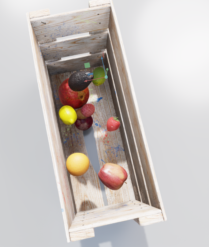
This post shows you how to use a model to detect fruits packaged in a crate using synthetic data generated from NVIDIA Omniverse Replicator, an SDK that programmatically generates physically accurate 3D synthetic data. You can fine-tune a simple pretrained model with this data, instead of collecting real-world data. Using synthetic data, you can create the exact scene you want, and even add new elements or adjust the scene, further iterating on the object detection pipeline.
Build the dataset
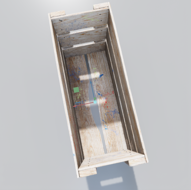
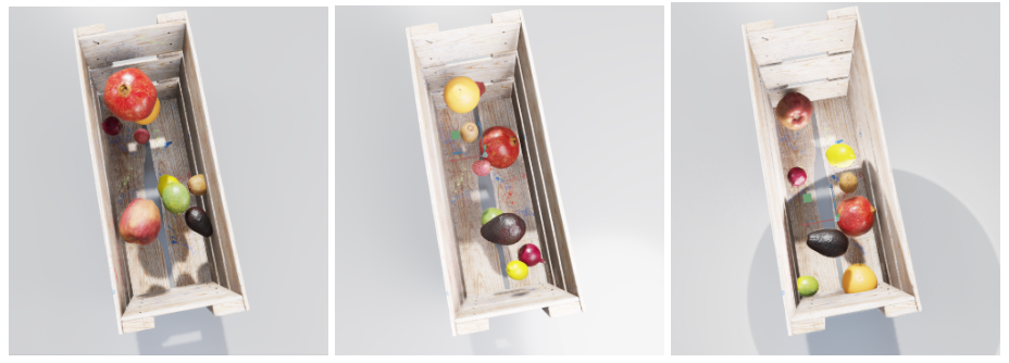
To generate the synthetic data, start by creating your environment in the digital world. For the example presented here, the environment is a surface that is consistent across all the generated data.
In this section, you are using NVIDIA Omniverse Code to run the replicator script. The following screenshots are pulled from the NVIDIA Omniverse Code GUI. After completing the script, you can continue to run within NVIDIA Omniverse Code to see the data as it is generated, or you can run in your local terminal in a headless mode. Both methods will be described.
To this end, load three Universal Scene Description (USD) assets that are included in NVIDIA Omniverse to create the basic scene using the following code:
with rep.new_layer():
    CRATE = 'omniverse://localhost/NVIDIA/Samples/Marbles/assets/standalone/SM_room_crate_3/SM_room_crate_3.usd'
    SURFACE = 'omniverse://localhost/NVIDIA/Assets/Scenes/Templates/Basic/display_riser.usd'
    ENVS = 'omniverse://localhost/NVIDIA/Assets/Scenes/Templates/Interior/ZetCG_ExhibitionHall.usd'
After loading these assets, set them as static elements in the scene using the NVIDIA Omniverse Replicator API. Create NVIDIA Omniverse Replicator elements from the loaded USDs and give the fruit crate a position and weight on top of the ground. To have the crate sit on top of the surface, make both physics colliders so one does not “fall through” the other:
env = rep.create.from_usd(ENVS)
    surface = rep.create.from_usd(SURFACE)
    with surface:
        rep.physics.collider()
    crate = rep.create.from_usd(CRATE)
    with crate:
        rep.physics.collider()
        rep.physics.mass(mass=10000)
        rep.modify.pose(
                position=(0, 20, 0),
                rotation=(0, 0, 90)
            )
Next, load the fruit USD assets, this time storing them in a dictionary with their class name as a key and the asset location as a value. With this approach, you can iterate through them later.
FRUIT_PROPS = {
        'apple': 'omniverse://localhost/NVIDIA/Assets/ArchVis/Residential/Food/Fruit/Apple.usd',
        'avocado': 'omniverse://localhost/NVIDIA/Assets/ArchVis/Residential/Food/Fruit/Avocado01.usd',
        'kiwi': 'omniverse://localhost/NVIDIA/Assets/ArchVis/Residential/Food/Fruit/Kiwi01.usd',
        'lime': 'omniverse://localhost/NVIDIA/Assets/ArchVis/Residential/Food/Fruit/Lime01.usd',
        'lychee': 'omniverse://localhost/NVIDIA/Assets/ArchVis/Residential/Food/Fruit/Lychee01.usd',
        'pomegranate': 'omniverse://localhost/NVIDIA/Assets/ArchVis/Residential/Food/Fruit/Pomegranate01.usd',
        'onion': 'omniverse://localhost/NVIDIA/Assets/ArchVis/Residential/Food/Vegetables/RedOnion.usd',
        'lemon': 'omniverse://localhost/NVIDIA/Assets/ArchVis/Residential/Decor/Tchotchkes/Lemon_01.usd',
        'orange': 'omniverse://localhost/NVIDIA/Assets/ArchVis/Residential/Decor/Tchotchkes/Orange_01.usd'    }
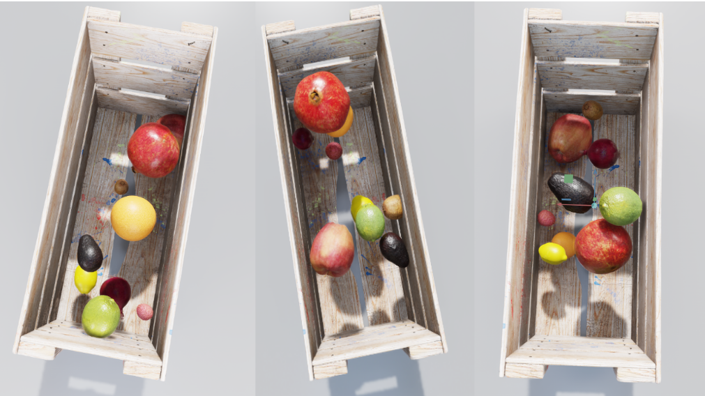
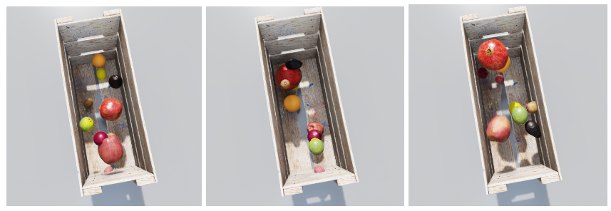
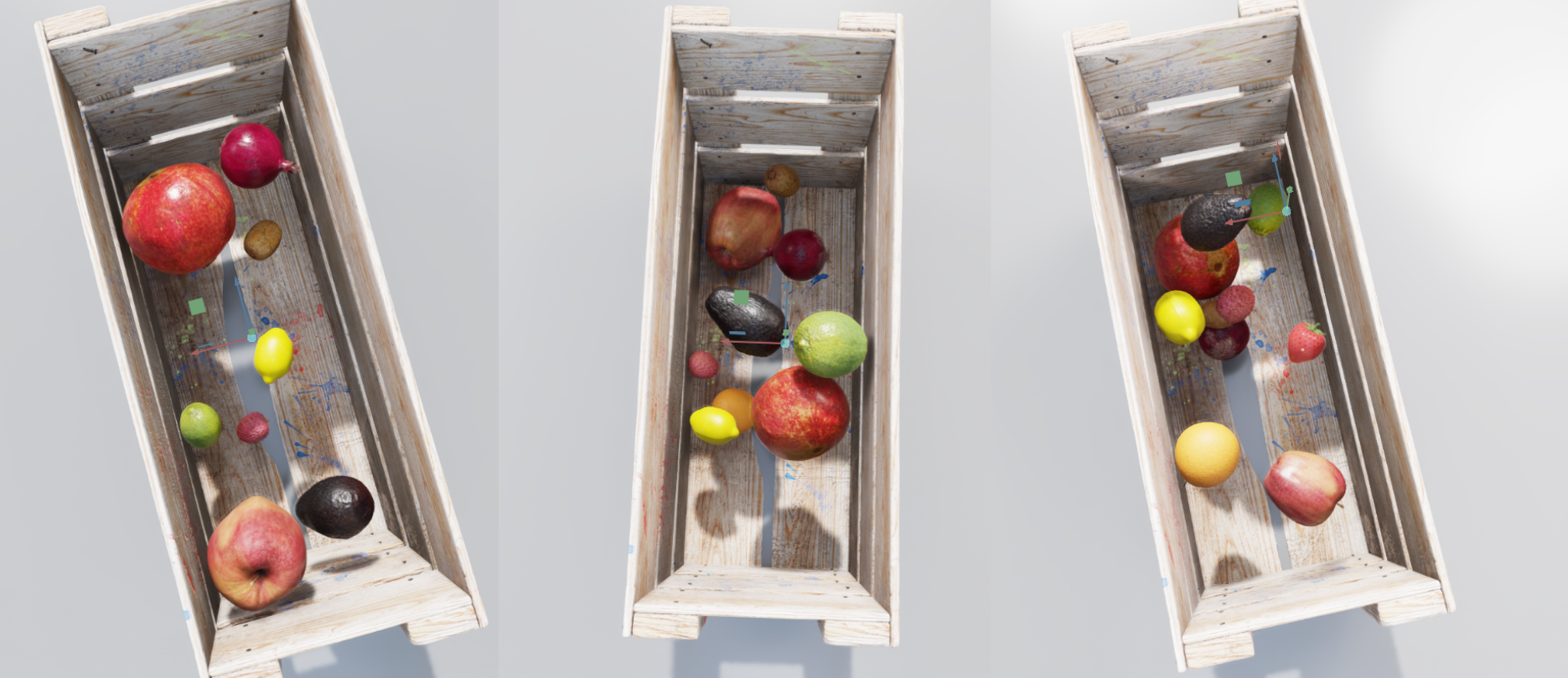
To generate data that is distinct in each frame, randomize the fruits that appear in each frame, where the fruits appear in the crate, and the total number of fruits. This gives the most coverage of each configuration of fruit that might be seen in an actual manufacturing line.
def random_props(file_name, class_name, max_number=1, one_in_n_chance=3):
        instances = rep.randomizer.instantiate(file_name, size=max_number, mode='scene_instance')
        print(file_name)
        with instances:
            rep.modify.semantics([('class', class_name)])
            rep.modify.pose(
                position=rep.distribution.uniform((-8, 5, -25), (8, 30, 25)),
                rotation=rep.distribution.uniform((-180,-180, -180), (180, 180, 180)),
                scale = rep.distribution.uniform((0.8), (1.2)),
            )

            rep.modify.visibility(rep.distribution.choice([True],[False]*(one_in_n_chance)))
        return instances.node
To further diversify the dataset, introduce some other randomization to each frame. Start by randomizing the number, color, and amount of light for each frame using the following code:
def sphere_lights(num):
        lights = rep.create.light(
            light_type="Sphere",
            temperature=rep.distribution.normal(6500, 500),
            intensity=rep.distribution.normal(30000, 5000),
            position=rep.distribution.uniform((-300, -300, -300), (300, 300, 300)),
            scale=rep.distribution.uniform(50, 100),
            count=num        )
        return lights.node
    rep.randomizer.register(sphere_lights)
Camera angle is another variation to introduce into the scene to account for different positions of the crate and camera heights. The code below also ensures that the camera is always facing the position of the crate, even as its position is adjusted.
with camera:
            rep.modify.pose(position=rep.distribution.uniform((-10, 105, -20), (5, 120, -5)), look_at=(0,20,0))
The final step is running the data generation script and recording the desired information. For this example, write out the baseline RGB data, bounding boxes, and labels for the fruit in each frame produced.
with rep.trigger.on_frame(num_frames=10):
        for n, f in FRUIT_PROPS.items():
            random_props(f, n)

        rep.randomizer.sphere_lights(5)

    # Initialize and attach writer
    writer = rep.WriterRegistry.get("BasicWriter")
    writer.initialize(output_dir="fruit_data", rgb=True, bounding_box_2d_tight=True)
    writer.attach([render_product])
After the NVIDIA Omniverse Replicator script is created, there are two ways to generate the full dataset. The preceding images are stills from the NVIDIA Omniverse Code GUI, which enables you to adjust the scene and immediately visualize the changes. This GUI gives you the chance to visualize the data at every code change you make. Once you are content with the script, generate a full dataset of many more images.
The next steps detail how you can either continue to run your code in the Script Editor of the NVIDIA Omniverse Code GUI or run it completely in your own local terminal.
To run the headless script, add the following line to the end of the existing script:
rep.orchestrator.runTo run this code headless inside the NVIDIA Omniverse container, first locate the omni.code.replicator.sh script. Open the NVIDIA Omniverse Launcher and navigate to the Code app. Click the menu to the right of the launch button to see the location of your NVIDIA Omniverse Code install. From that folder, you can run the following command, passing in the location of your own headless script:
./omni.code.replicator.sh --no-window --/omni/replicator/script="FruitBasketOVEReplicatorDemo/data_generation/generate_data_headless.py"
Explore your data
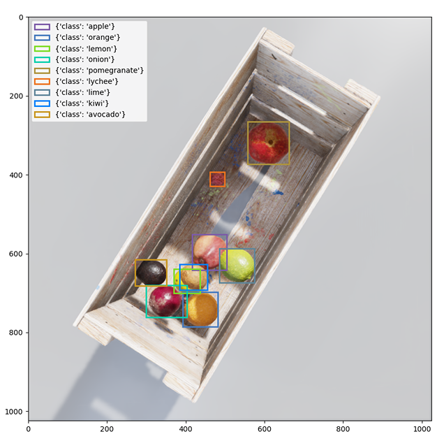
After you have created your first frames using the Replicator script, you can tune the parameters to get the desired output. To do this, you may want to see the bounding boxes placed on the generated images.
Functions within NVIDIA Omniverse are created to visualize the color and labels of bounding box data on generated images. These functions take in the path to the generated image for the background, bounding box data, class labels, and the place to store the visualization with a colorized bounding box.
def colorize_bbox_2d(rgb_path, data, id_to_labels, file_path):

    rgb_img = Image.open(rgb_path)
    colors = [data_to_colour(bbox["semanticId"]) for bbox in data]
    fig, ax = plt.subplots(figsize=(10, 10))
    ax.imshow(rgb_img)
    for bbox_2d, color, index in zip(data, colors, range(len(data))):
        labels = id_to_labels[str(index)]
        rect = patches.Rectangle(
            xy=(bbox_2d["x_min"], bbox_2d["y_min"]),
            width=bbox_2d["x_max"] - bbox_2d["x_min"],
            height=bbox_2d["y_max"] - bbox_2d["y_min"],
            edgecolor=color,
            linewidth=2,
            label=labels,
            fill=False,
        )
        ax.add_patch(rect)

    plt.legend(loc="upper left")

    plt.savefig(file_path)
To use the function as it appears above, run the following commands, using the data generated:
bbox2d_loose_file_name = "bounding_box_2d_tight_0.npy"
data = np.load(os.path.join(out_dir, bbox2d_tight_file_name))

bbox2d_tight_labels_file_name = "bounding_box_2d_tight_labels_0.json"
with open(os.path.join(out_dir, bbox2d_tight_labels_file_name), "r") as json_data:
    bbox2d_loose_id_to_labels = json.load(json_data)

colorize_bbox_2d(rgb_path, data, bbox2d_loose_id_to_labels, os.path.join(vis_out_dir, "bbox2d_tight.png"))
Train your model
After generating your data, you can start the model training workflow. This example uses the PyTorch torchvision package to fine-tune a pretrained Faster R-CNN model. However, synthetic data can also be introduced into other pipelines that use tools like NVIDIA TAO Toolkit or TensorFlow.
The first step in the training script is to define the dataset to build the PyTorch DataLoader. Do some preliminary work to sort the three file types and correlate the bounding box information with the correct fruit label. The key output here is the target that has the bounding box information, fruit labels, box areas, and the image ID.
target = {}
        target["boxes"] = torch.as_tensor(boxes, dtype=torch.float32)
        target["labels"] = torch.as_tensor(labels_out, dtype=torch.int64)
        target["image_id"] = torch.tensor([idx])
        target["area"] = area
Once you have the dataset, split the data into training, validation, and test sections for the training pipeline. Then create a data loader for the training and validation datasets using the following code:
data_loader = torch.utils.data.DataLoader(
dataset, batch_size=16, shuffle=True, num_workers=4,
collate_fn= collate_fn)
validloader = torch.utils.data.DataLoader(
valid, batch_size=16, shuffle=True, num_workers=4,
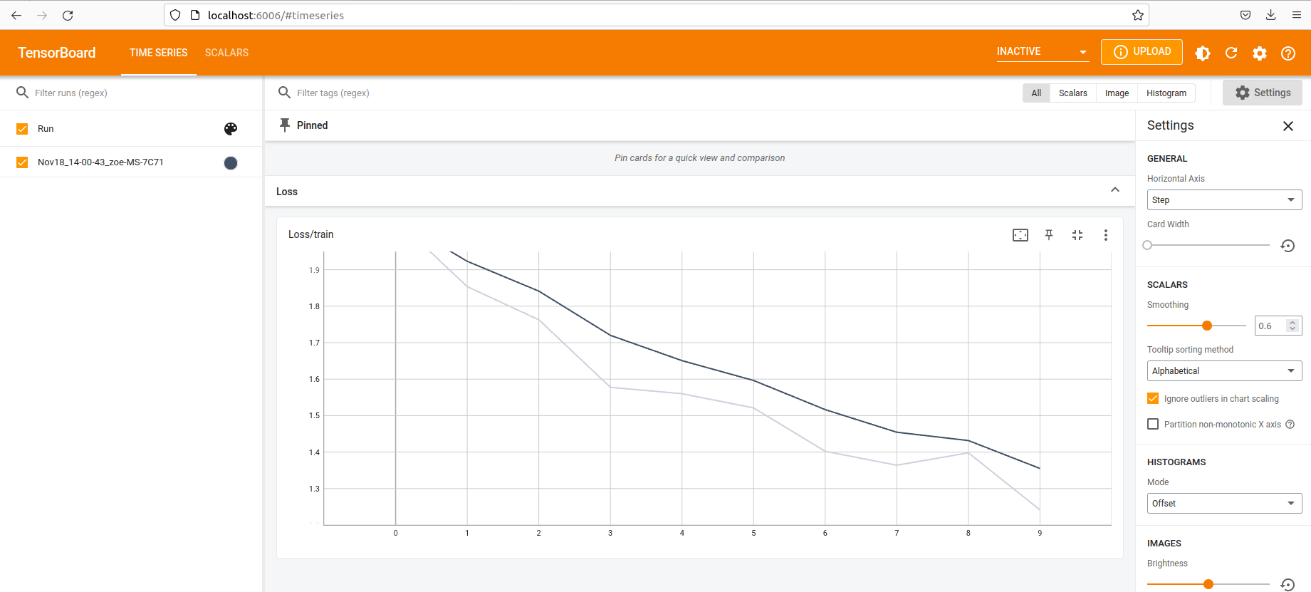
collate_fn= collate_fn) With the dataset and data loader configured, continue training. Track loss over each epoch and configure the data to show in TensorBoard for visualization.
params = [p for p in model.parameters() if p.requires_grad]
    optimizer = torch.optim.SGD(params, lr=0.001)
    len_dataloader = len(data_loader)
    model.train()
    for epoch in range(num_epochs):
        optimizer.zero_grad()

        i = 0
        for imgs, annotations in data_loader:
            i += 1
            imgs = list(img.to(device) for img in imgs)
            annotations = [{k: v.to(device) for k, v in t.items()} for t in annotations]
            loss_dict = model(imgs, annotations)
            losses = sum(loss for loss in loss_dict.values())
            writer.add_scalar("Loss/train", losses, epoch)

            losses.backward()
            optimizer.step()

            print(f'Iteration: {i}/{len_dataloader}, Loss: {losses}')
When you have the loss sufficiently reduced and are happy with how the model has trained, save the model. The final step is deploying the model to production.
Deploy your model to production
First, use NVIDIA Triton Inference Server to export the model to an ONNX format using the following script:
torch.onnx.export(model,
                    dummy_input,
                    os.path.join(OUTPUT_DIR, "model.onnx"),
                    opset_version=11,
                    input_names=["input"],
                    output_names=["boxes", "labels", "scores", "masks"]
                    )
Next, run the NVIDIA Triton container from NGC, then start the server with the following command:
tritonserver --model-repository=/model_repository --model-control-mode explicit --exit-on-error 0 --repository-poll-secs 3Using NVIDIA Triton, you can “poll” a model repository to see if a change has occurred. Then, copy the model into the model_repository directory.
Next, copy the model into the NVIDIA Triton directory with bash using the following code:
mkdir model_repository/dmcount_onnx/ # create the folder with the model name
mkdir model_repository/dmcount_onnx/1/ # create the folder for the model version
cp model.onnx model_repository/dmcount_onnx/1/ # move the file to the directory
Now it is time for inference.
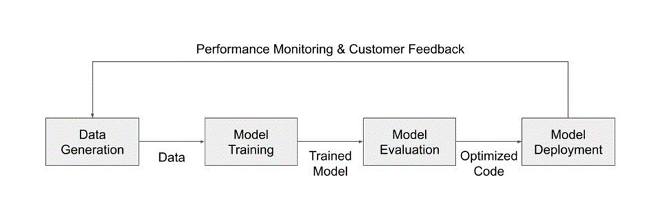
Complete the cycle
After deploying the model, you can choose to iterate further on this first full implementation of the object detection pipeline. If you choose to add to the original dataset, you can do so with relatively little overhead.
For example, to add a new fruit (strawberry) to the original set of options, load the new asset to the original dictionary and generate the new data:
'strawberry': 'omniverse://localhost/NVIDIA/Assets/ArchVis/Residential/Food/Berries/strawberry.usd',In the training step, adjust the label mapping to fit the addition of the strawberry to the data:
static_labels = {
            'apple' : 0,
            'avocado' : 1,
            'kiwi' : 2,
            'lime' : 3,
            'lychee' : 4,
            'pomegranate' : 5,
            'onion' : 6,
            'strawberry' : 7,
            'lemon' : 8,
            'orange' : 9,
        }
You can now visualize the bounding box data as before, noticing the addition of the strawberry to some of the frames generated. The other elements of the pipeline remain the same. In the production deployment, the strawberry appears correctly annotated.
Introducing new data to the object detection pipeline is streamlined when using synthetic data, which makes deploying to production a goal within reach. Synthetic data unlocks the full potential of an iterative training workflow.
When you can easily modify, tune, and generate massive amounts of data, you are no longer bottlenecked by the first step of the training pipeline and can focus on fine-tuning and pushing the model to production.
Summary
This tutorial has shown how to integrate synthetic data into your already existing models. The first step shows how NVIDIA Omniverse Code gives you an interactive GUI for writing your own Replicator script. This script can be customized to your scene and data preferences required for the model. You can then create the prelabeled data to your exact specification. From there, you can take the synthetic data to wherever you want. The example in this post integrates the data to a TorchVision pipeline for fine-tuning.
The last step of this process is to deploy your trained model to NVIDIA Triton for inference. This workflow is representative of all the options you have when you integrate synthetic data into your existing workflows. NVIDIA Omniverse Replicator gives you a tool to iteratively generate your synthetic data to fit into your existing workflows.
To get started with Omniverse Replicator, download NVIDIA Omniverse and install the NVIDIA Omniverse Code app. To access the code and other Omniverse Replicator synthetic data examples, visit NVIDIA-Omniverse/synthetic-data-examples on GitHub.
Additional resources
Want to learn more? Check out these expert-led NVIDIA GTC 2023 sessions on generating synthetic data and Omniverse Replicator.
For more information and the latest news, see the following resources:
- Visit Get Started Building on Omniverse for all the resources you need to learn how to build custom USD-based applications and extensions for the platform.
- Follow Omniverse on Instagram, Twitter, YouTube, and Medium for additional resources and inspiration.
- Check out the Omniverse forums and join our Discord Server and Twitch to chat with the community.
- Visit the NVIDIA-Omniverse GitHub repo to explore code samples and extensions built by the community.
