Accelerated Ray Tracing in One Weekend in CUDA

Recent announcements of NVIDIA’s new Turing GPUs, RTX technology, and Microsoft’s DirectX Ray Tracing have spurred a renewed interest in ray tracing. Using these technologies vastly simplifies the ability to write applications using ray tracing.

But what if you’re curious about how ray tracing actually works? One way to learn is to code your own ray tracing engine.  Would you like to build a ray tracer that runs on your GPU using CUDA? If so, this post is for you! You’ll learn more about CUDA programming as well as ray tracing in one fell swoop.

Peter Shirley has written a series of fantastic ebooks about Ray Tracing starting from coding the very basics in one weekend to deep topics to spend your life investigating. You can find out more about these books at http://in1weekend.blogspot.com/. The books are now free or pay-what-you-wish and 50% of the proceeds go towards not-for-profit programming education organizations. They are also available on Amazon as a Kindle download. You should sit down and read Ray Tracing in One Weekend before diving into the rest of this post. Each section of this post corresponds to one of the chapters from the book. Even if you don’t sit down and write your own ray tracer in C++, the core concepts should get you started with a GPU-based engine using CUDA.

Preliminaries

The C++ ray tracing engine in the One Weekend book is by no means the fastest ray tracer, but translating your C++ code to CUDA can result in a 10x or more speed improvement! Let’s walk through the process of converting the C++ code from Ray Tracing in One Weekend to CUDA. Note that as you go through the C++ coding process, consider using git tags or branches to allow you to go back to each chapter’s code easily. You can compare your C++ code with Peter Shirley’s at https://github.com/petershirley/raytracinginoneweekend. After trying your hand at using CUDA, you can also compare with my CUDA code at https://github.com/rogerallen/raytracinginoneweekendincuda. Be sure to use the branches I’ve created for each chapter. (E.g. git checkout ch12_where_next_cuda.)

This post assumes you understand a few of the basics of CUDA. If not, you can start with An Even Easier Introduction to CUDA here on the NVIDIA Developer Blog. You’ll need to have your development environment set up to compile and run CUDA code. We will also be profiling with nvprof, so you may want to familiarize yourself with how to profile your code with nvprof, too. The code in my repository was written using Ubuntu Linux and CUDA 9.x, but you should be able to adapt these instructions to recent CUDA releases on either Windows or MacOS, too.

If you start with my Makefile, note that I build for a GTX 1070 card using specific -gencode flags for that card (-gencode arch=compute_60,code=sm_60). You will want to adjust the architecture and feature settings for the GPU or GPUs you will be running on. In my Makefile, the main targets you will use are for building the executable make cudart and for running and creating the output image make out.ppm.

Please note that when the CUDA code runs for longer than a few seconds, you may notice error 6 (cudaErrorLaunchTimeout) and on Windows your screen may also black out for a few seconds. This is because your window manager thinks the GPU is malfunctioning when it doesn’t respond after a certain amount of time.  Linux users can take steps to resolve this issue via this post.

In this post, you’ll learn about the following:

• a Unified Memory frame buffer that is written by the GPU and read by the CPU
• launching rendering work on the GPU
• Writing C++ code that can run on either the CPU or GPU
• Checking for slower double precision floating point code.
• C++ Memory management. Allocating memory on the GPU and instantiating it at run time on the GPU.
• Per-thread random number generation with cuRAND.

First Image

Chapter 1 in Ray Tracing in One Weekend ends with generating an image with a simple gradient for red & green channels. In a serial language, you use nested for loops to iterate over all of the pixels. In CUDA, the scheduler takes blocks of threads and schedules them on the GPU. But, before we get to that, we have to set up a few preliminaries…

For clarity, we change main.cc to main.cu to let both us and the compiler know this is CUDA source.

Each CUDA API call we make returns an error code that we should check. We check the cudaError_t result with a checkCudaErrors macro to output the error to stdout before we reset the CUDA device and exit. For help with any errors, see the cudaError_t enum section of https://docs.nvidia.com/cuda/cuda-runtime-api/group__CUDART__TYPES.html for what each error code means.

#define checkCudaErrors(val) check_cuda( (val), #val, __FILE__, __LINE__ )
void check_cuda(cudaError_t result, char const *const func, const char *const file, int const line) {
    if (result) {
        std::cerr << "CUDA error = " << static_cast<unsigned int>(result) << " at " <<
        file << ":" << line << " '" << func << "' \n";
        // Make sure we call CUDA Device Reset before exiting
        cudaDeviceReset();
        exit(99);
    }
}

We allocate an nx*ny image-sized frame buffer (FB) on the host to hold the RGB float values calculated by the GPU, allowing communication between the CPU and GPU. cudaMallocManaged allocates Unified Memory, which allows us to rely on the CUDA runtime to move the frame buffer on demand to the GPU for the rendering and back to the CPU for outputting the PPM image.  Using cudaDeviceSynchronize lets the CPU know when the GPU is done rendering.

int num_pixels = nx*ny;
size_t fb_size = 3*num_pixels*sizeof(float);

// allocate FB
float *fb;
checkCudaErrors(cudaMallocManaged((void **)&fb, fb_size));

This call renders the image on the GPU and has the CUDA runtime divide the work on the GPU into blocks of 8×8 threads. You might also try other thread sizes to what works best for your machine. I tried to find a block size that:
(1) is a small, square region so the work would be similar.  This should help each pixel do a similar amount of work. If some pixels work much longer than other pixels in a block, the efficiency of that block is impacted.
(2) has a pixel count that is a multiple of 32 in order to fit into warps evenly.

    int tx = 8;
    int ty = 8;
    ...
    // Render our buffer
    dim3 blocks(nx/tx+1,ny/ty+1);
    dim3 threads(tx,ty);
    render<<<blocks, threads>>>(fb, nx, ny);
    checkCudaErrors(cudaGetLastError());
    checkCudaErrors(cudaDeviceSynchronize());

Because of the way the book’s code is written, I didn’t choose to convert the final float values to 8-bit components on the GPU. As a further performance improvement, you could also choose to have the GPU convert the final float values to 8-bit components, saving bandwidth when the data is read back.

Threads launch in blocks and each block has 64 threads running the kernel function render (note the __global__ identifier). Using the threadIdx and blockIdx CUDA built-in variables we identify the coordinates of each thread in the image (i,j) so it knows how to calculate the final color. It is possible with images of sizes that are not multiples of the block size to have extra threads running that are outside the image. We must make sure these threads do not try to write to the frame buffer and return early.

Aside from that, the image calculation is very similar to the standard C++ code.

__global__ void render(float *fb, int max_x, int max_y) {
    int i = threadIdx.x + blockIdx.x * blockDim.x;
    int j = threadIdx.y + blockIdx.y * blockDim.y;
    if((i >= max_x) || (j >= max_y)) return;
    int pixel_index = j*max_x*3 + i*3;
    fb[pixel_index + 0] = float(i) / max_x;
    fb[pixel_index + 1] = float(j) / max_y;
    fb[pixel_index + 2] = 0.2;
}

Back on the host, after the cudaDeviceSynchronize we can access the frame buffer on the CPU host to output the image to stdout.

    // Output FB as Image
    std::cout << "P3\n" << nx << " " << ny << "\n255\n";
    for (int j = ny-1; j >= 0; j--) {
        for (int i = 0; i < nx; i++) {
            size_t pixel_index = j*3*nx + i*3;
            float r = fb[pixel_index + 0];
            float g = fb[pixel_index + 1];
            float b = fb[pixel_index + 2];
            int ir = int(255.99*r);
            int ig = int(255.99*g);
            int ib = int(255.99*b);
            std::cout << ir << " " << ig << " " << ib << "\n";
        }
    }
    checkCudaErrors(cudaFree(fb));

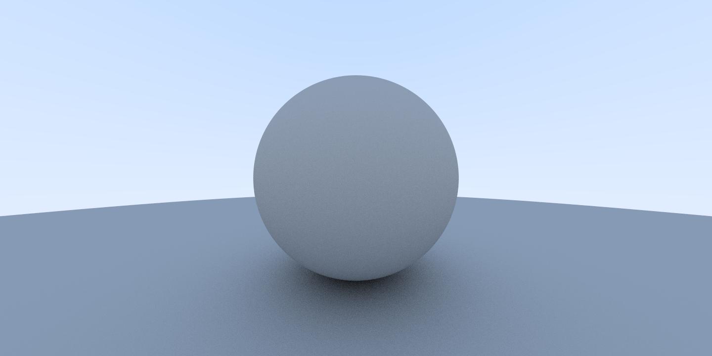
We also cudaFree the frame buffer when we are finished with it. You can compare your code with mine here. With that you should produce a very similar result to your C++ program, with an example shown in figure 1. On Linux, there are many ways to view PPM images including the default viewer on Ubuntu (eog) which can view the PPM text output: eog out.ppm.

Adding Vectors

Chapter 2 in Ray Tracing in One Weekend introduce a vector class that can be used on both the CPU & GPU. To allow this, we annotate all of the vec3 class member functions with __host__ __device__ keywords so we can execute them on the GPU and CPU.

class vec3  {
public:
     __host__ __device__ vec3() {}
     __host__ __device__ vec3(float e0, float e1, float e2) { e[0] = e0; e[1] = e1; e[2] = e2; }
     __host__ __device__ inline float x() const { return e[0]; }
     __host__ __device__ inline float y() const { return e[1]; }
     __host__ __device__ inline float z() const { return e[2]; }
...

Use these __host__ __device__ keywords before all methods except the operator>> and operator<< methods.

Given this class, you can update your main.cu code to access an FB made up of vec3 instead of 3 floats, similar to the C++ code. The end result shown in figure 2 should still look like figure 1. See the Chapter 2 reference implementation if you have any troubles.

Classing Up the GPU

The rest of the C++ classes introduced in the book only get used on the GPU, so I annotate them with just __device__ keywords. In Chapter 3, the book introduces the ray class.

class ray
{
   public:
      __device__ ray() {}
      __device__ ray(const vec3& a, const vec3& b) { A = a; B = b; }
      __device__ vec3 origin() const       { return A; }
      __device__ vec3 direction() const    { return B; }
      __device__ vec3 point_at_parameter(float t) const { return A + t*B; }

      vec3 A;
      vec3 B;
};

You will also need to add the __device__ keyword to the color function since that is called from the render kernel.

We need to be careful to check for double precision code. Current GPUs run fastest when they do calculations in single precision. Double precision calculations can be several times slower on some GPUs. For example, this may look like a single precision calculation:

float t = 0.5*(unit_direction.y() + 1.0);

But, this code will calculate the multiplication and addition at double precision. While the unit_direction.y() result is float, since the floating-point constants 0.5 and 1.0 are doubles the float value is upconverted to double for the math. Only when the result is written into t will it be converted to single precision. To force single precision math, you need to coerce those constants to float. I typically add an “f” as a suffix. Note that the vec3() constructors coerce the values to float without any calculations, so you don’t need to change those.

__device__ vec3 color(const ray& r) {
   vec3 unit_direction = unit_vector(r.direction());
   float t = 0.5f*(unit_direction.y() + 1.0f);
   return (1.0f-t)*vec3(1.0, 1.0, 1.0) + t*vec3(0.5, 0.7, 1.0);
}

__global__ void render(vec3 *fb, int max_x, int max_y, vec3 lower_left_corner, vec3 horizontal, vec3 vertical, vec3 origin) {
   int i = threadIdx.x + blockIdx.x * blockDim.x;
   int j = threadIdx.y + blockIdx.y * blockDim.y;
   if((i >= max_x) || (j >= max_y)) return;
   int pixel_index = j*max_x + i;
   float u = float(i) / float(max_x);
   float v = float(j) / float(max_y);
   ray r(origin, lower_left_corner + u*horizontal + v*vertical);
   fb[pixel_index] = color(r);
}

It is very easy to miss a double precision constant. For the most accurate test, use nvprof. For example:

nvprof --metrics inst_fp_32,inst_fp_64 ./cudart > out.ppm

This will output a report similar to the following:

Rendering a 200x100 image in 8x8 blocks.
==21852== NVPROF is profiling process 21852, command: ./cudart
took 0.103823 seconds.
==21852== Profiling application: ./cudart
==21852== Profiling result:
==21852== Metric result:
Invocations                                   Metric Name                            Metric Description             Min             Max             Avg
Device "GeForce GTX 1070 (0)"
Kernel: render(vec3*, int, int, vec3, vec3, vec3, vec3)
1                                    inst_fp_32                       FP Instructions(Single)         1577600         1577600         1577600
1                                    inst_fp_64                       FP Instructions(Double)               0               0               0

This shows many single precision (inst_fp_32) and zero double precision (inst_fp_64) instructions. If you see any double precision instructions running on the GPU, you will not achieve the best performance.

Note that when running nvprof, you can temporarily change the size of your output image to make it smaller. This should make nvprof run very fast.

My code for this section can be found here.

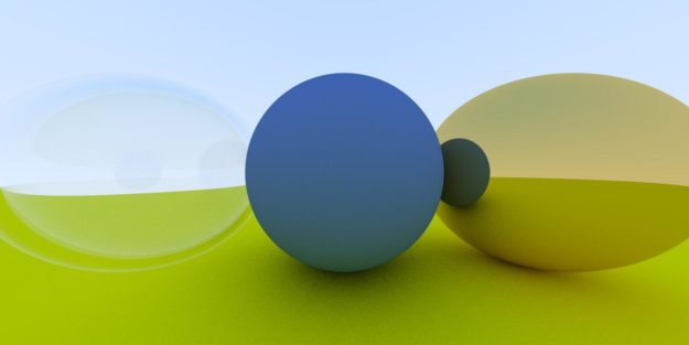
Hit the Sphere

Chapter 4 uses concepts we’ve introduced above. There is a hit_sphere routine that is called from the GPU, so it requires a __device__ annotation. In it, there are floating-point constants and math to attend to, too. The output should resemble figure 3.

See the Chapter 4 reference implementation if you have any troubles.

Manage Your Memory

The new topic introduces how we handle memory management for CUDA C++ classes on CPU & GPU. We are going to allocate our scene’s objects on the GPU and this requires two pieces of code. First,  we allocate a d_list of hitables and a d_world to hold those objects in the main routine on the CPU. (The d_ prefix is for device-only data.) Next, we call a create_world kernel to construct those objects.

    hitable **d_list;
checkCudaErrors(cudaMalloc((void **)&d_list, 2*sizeof(hitable *)));
   hitable **d_world;
   checkCudaErrors(cudaMalloc((void **)&d_world, sizeof(hitable *)));
   create_world<<<1,1>>>(d_list,d_world);
   checkCudaErrors(cudaGetLastError());
   checkCudaErrors(cudaDeviceSynchronize());

In the kernel we make sure to only execute the construction of the world once

__global__ void create_world(hitable **d_list, hitable **d_world) {
    if (threadIdx.x == 0 && blockIdx.x == 0) {
        *(d_list)   = new sphere(vec3(0,0,-1), 0.5);
        *(d_list+1) = new sphere(vec3(0,-100.5,-1), 100);
        *d_world    = new hitable_list(d_list,2);
    }
}

To use this world, we pass it to our render kernel and color function, along with the values describing our camera

render<<<blocks, threads>>>(fb, nx, ny,
                            vec3(-2.0, -1.0, -1.0),
                            vec3(4.0, 0.0, 0.0),
                            vec3(0.0, 2.0, 0.0),
                            vec3(0.0, 0.0, 0.0),
                            d_world);

And the kernels…

__global__ void render(vec3 *fb, int max_x, int max_y,vec3 lower_left_corner, vec3 horizontal, vec3 vertical, vec3 origin, hitable **world)
{
   int i = threadIdx.x + blockIdx.x * blockDim.x;
   int j = threadIdx.y + blockIdx.y * blockDim.y;
   if((i >= max_x) || (j >= max_y)) return;
   int pixel_index = j*max_x + i;
   float u = float(i) / float(max_x);
   float v = float(j) / float(max_y);
   ray r(origin, lower_left_corner + u*horizontal + v*vertical);
   fb[pixel_index] = color(r, world);
}

__device__ vec3 color(const ray& r, hitable **world) {
   hit_record rec;
   if ((*world)->hit(r, 0.0, FLT_MAX, rec)) {
      return 0.5f*vec3(rec.normal.x()+1.0f, rec.normal.y()+1.0f, rec.normal.z()+1.0f);
   }
   else {
      vec3 unit_direction = unit_vector(r.direction());
      float t = 0.5f*(unit_direction.y() + 1.0f);
      return (1.0f-t)*vec3(1.0, 1.0, 1.0) + t*vec3(0.5, 0.7, 1.0);
   }
}

After we’re done, what we construct, we must delete; at the end of main you can see:

checkCudaErrors(cudaDeviceSynchronize());
free_world<<<1,1>>>(d_list,d_world);
checkCudaErrors(cudaGetLastError());
checkCudaErrors(cudaFree(d_list));
checkCudaErrors(cudaFree(d_world));
checkCudaErrors(cudaFree(fb));

And the free_world kernel is just:

__global__ void free_world(hitable **d_list, hitable **d_world) {
   delete *(d_list);
   delete *(d_list+1);
   delete *d_world;
}

In addition, there are hitable.h, hitable_list.h, and sphere.h files which all have classes and methods that are called from the GPU, so they require __device__ annotations. Finally, there are floating-point constants and math to attend to, too. Figure 4 shows what your code should be generating.

My code for this section lies here.

It’s All Random

Chapter 6 introduces stochastic or randomly determined values. Random numbers are a special topic for CUDA and requires the cuRAND library. Since “random numbers” on a computer actually consist of pseudorandom sequences, we need to setup and remember state for every thread on the GPU.

To do that we create a d_rand_state object for every pixel in our main routine.

#include <curand_kernel.h>
...
   curandState *d_rand_state;
   checkCudaErrors(cudaMalloc((void **)&d_rand_state, num_pixels*sizeof(curandState)));
...
   render_init<<<blocks, threads>>>(nx, ny, d_rand_state);
   checkCudaErrors(cudaGetLastError());
   checkCudaErrors(cudaDeviceSynchronize());
   render<<<blocks, threads>>>(fb, nx, ny,  ns, d_camera, d_world, d_rand_state);
   checkCudaErrors(cudaGetLastError());
   checkCudaErrors(cudaDeviceSynchronize());

We initialize rand_state for every thread. For performance measurement, I wanted to be able to separate the time for random initialization from the time it takes to do the rendering, so I made this a separate kernel. You might also choose to do this initialization at the start of your render kernel.

__global__ void render_init(int max_x, int max_y, curandState *rand_state) {
   int i = threadIdx.x + blockIdx.x * blockDim.x;
   int j = threadIdx.y + blockIdx.y * blockDim.y;
   if((i >= max_x) || (j >= max_y)) return;
   int pixel_index = j*max_x + i;
   //Each thread gets same seed, a different sequence number, no offset
   curand_init(1984, pixel_index, 0, &rand_state[pixel_index]);
}

And finally, we pass it into our render kernel, make a local copy and use it per-thread.  Replacing any drand48() calls with curand_uniform(&local_rand_state).

__global__ void render(vec3 *fb, int max_x, int max_y, int ns, camera **cam, hitable **world, curandState *rand_state) {
   int i = threadIdx.x + blockIdx.x * blockDim.x;
   int j = threadIdx.y + blockIdx.y * blockDim.y;
   if((i >= max_x) || (j >= max_y)) return;
   int pixel_index = j*max_x + i;
   curandState local_rand_state = rand_state[pixel_index];
   vec3 col(0,0,0);
   for(int s=0; s < ns; s++) {
      float u = float(i + curand_uniform(&local_rand_state)) / float(max_x);
      float v = float(j + curand_uniform(&local_rand_state)) / float(max_y);
      ray r = (*cam)->get_ray(u,v);
      col += color(r, world);
   }
   fb[pixel_index] = col/float(ns);
}

Note that now using debug flags in compilation makes a big difference in runtime. If you have those flags set on your compilation command line, remove them for a significant speedup. The image should resemble that shown in figure 4, earlier, but run faster.

My code for this chapter is here.

Iteration vs. Recursion

The default translation of the color function results in a stack overflow since it can call itself many times. But, the code can be simply be translated into a loop instead of recursion. In fact, later code in the book puts a limit of 50 levels of recursion, so we’re just adding that limit a few chapters early.

The original C++ code looks like this and you can see if the world->hit returns true, the function recurs.

vec3 color(const ray& r, hitable *world) {
   hit_record rec;
   if (world->hit(r, 0.001, MAXFLOAT, rec)) {
      vec3 target = rec.p + rec.normal + random_in_unit_sphere();
      return 0.5*color( ray(rec.p, target-rec.p), world);
   }
   else {
      vec3 unit_direction = unit_vector(r.direction());
      float t = 0.5*(unit_direction.y() + 1.0);
      return (1.0-t)*vec3(1.0, 1.0, 1.0) + t*vec3(0.5, 0.7, 1.0);
   }
}

And I translated that into the following for CUDA:

__device__ vec3 color(const ray& r, hitable **world, curandState *local_rand_state) {
   ray cur_ray = r;
   float cur_attenuation = 1.0f;
   for(int i = 0; i < 50; i++) {
      hit_record rec;
      if ((*world)->hit(cur_ray, 0.001f, FLT_MAX, rec)) {
         vec3 target = rec.p + rec.normal + random_in_unit_sphere(local_rand_state);
         cur_attenuation *= 0.5f;
         cur_ray = ray(rec.p, target-rec.p);
      }
      else {
           vec3 unit_direction = unit_vector(cur_ray.direction());
           float t = 0.5f*(unit_direction.y() + 1.0f);
           vec3 c = (1.0f-t)*vec3(1.0, 1.0, 1.0) + t*vec3(0.5, 0.7, 1.0);
           return cur_attenuation * c;
        }
      }
   return vec3(0.0,0.0,0.0); // exceeded recursion
}

My code for this chapter is here.

The Rest of the Chapters

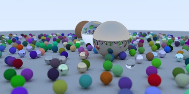
Chapters 8-12 use the same concepts we went over above to create the final image. You’ve learned all the concepts you need to finish the book. You should be able to take your C++ code, add the appropriate __device__ annotations, add appropriate delete or cudaFree calls, adjust any floating point constants and plumb the local random state as needed to complete the translation. The images that follow show what your code should generate assuming you convert your code to CUDA correctly.

See the reference implementation code if you have any troubles.

Here is my code for Chapter 8.

Here is my code for Chapter 9.

Here is my code for Chapter 10.

Here is my code for Chapter 11.

And finally, here is my code for the final chapter, Chapter 12. At this point, I hope you take a moment to compare the speedup from C++ to CUDA. My personal machine with a 6-core i7 takes about 90 seconds to render the C++ image.  To give some concrete examples for the speedup you might see, on a Geforce GTX 1070, this runs in 6.7 seconds for a 13x speedup.  Using a new GeForce RTX 2080, the image renders in just 4.7 seconds for a 19x speedup!  What speedup do you see?  When you try on your machine, be sure to try a range of thread block sizes (tx and ty in main.cu) to see if that helps your performance.

Next

I hope you enjoyed this walkthrough and it helps you in the process of creating a CUDA ray tracer. This is only a simple and relatively direct translation from C++ to CUDA. We didn’t try any further acceleration techniques and yet achieved up to a 19x speedup.  This is just the start on a journey you might enjoy for a long time–ray tracing is a deeply interesting subject. Here are a few more ideas to consider…

• continue reading the rest of the Peter Shirley’s series: Ray Tracing: The Next Week, and Ray Tracing: The Rest of Your Life.
• look into using the OptiX API which uses CUDA as the shading language, has CUDA interoperability and accesses the latest Turing RT Cores for hardware acceleration.
• Microsoft has announced DirectX 3D Ray Tracing, and NVIDIA has announced new hardware to take advantage of it–so perhaps now might be a time to look at real-time ray tracing?
• do you have multiple GPUs?  Consider adding even more parallelism by using them!

Acknowledgements

I would like to thank Mark Harris, Peter Shirley, Pawel Tabaszewski and Loyd Case for their helpful insights and encouragement in creating this post. I would also like to thank github user pfranz for making the first github repo with a tag for each chapter which was very handy.