Python is no stranger to data scientists. It ranks as the most popular computer language and is widely used for all kinds of tasks. Though Python is notoriously slow when the code is interpreted at runtime, many popular libraries make it run efficiently on GPUs for certain data science work. For example, popular deep learning frameworks such as TensorFlow, and PyTorch help AI researchers to efficiently run experiments. However, in certain domains like portfolio optimization, there are no Python libraries for easy acceleration of computational work. Developers must implement the algorithms from scratch to accelerate on the GPU.
In this post, we will show how we used Numba and Dask to accelerate a portfolio construction algorithm by 800x as introduced in a previous blog.
Introducing the Tooling + Use Case
Numba is a Python library that eases the implementation of GPU algorithms with Python. The Python GPU kernels can be Just in Time (JIT) compiled to run on the GPU. It makes writing CUDA more accessible to Python developers. For larger problems that don’t fit in a single GPU, we use Dask for distributed computation in a cluster of GPUs. Dask integrates well with Python libraries like Numpy, pandas, cuDF, CuPy, etc. It uses the same APIs and data structures so Python developers can pick it up easily.
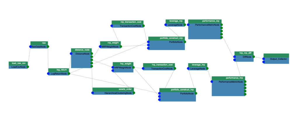
The portfolio construction algorithm is used to calculate the optimal weights for constructing portfolios. It is one of the most important steps that a fund manager has to do to manage assets. As shown in the Figure 1, the use case in the previous blog includes following steps:Load csv data of asset daily prices
- Run block bootstrap to generate 100k different scenarios.
- Compute the log returns for each scenario.
- Compute assets distances to run hierarchical clustering and Hierarchical Risk Parity (HRP) weights for the assets
- Compute the weights for the assets based on the Naïve Risk Parity (NRP) method.
- Compute the transaction cost based on weights adjustment on the rebalancing days.
- At every rebalancing date, calculate the portfolio leverage to reach the volatility target.
- Compute the Average annual Returns, STD Returns, Sharpe Ratios, Maximum Drawdown, and Calmar Ratio performance metrics for these two methods (HRP-NRP).
Figure 1: Computation graph for the portfolio construction algorithm.
There are quite a few steps involved in the preceding computation. To accelerate them on the GPU, the most important thing that we need to identify is the granularity of the parallelism.
Some of the steps, like the HRP algorithm, are serial in nature. It reorganizes the covariance matrix of the stock returns so similar investments are placed together. Then, it distributes the allocation through recursive bisection based on the cluster covariance. We might be able to vectorize a few steps of the HRP algorithm, however, the speed-up will be minimal because only a smaller number of parallel threads are used.
Since the generated scenarios are independent from each other and large in number, a better method of parallelism should be at the scenario level. The different scenarios are calculated using multiple GPU threads. We will describe in detail how to perform block bootstrapping calculations in a Numba GPU kernel.
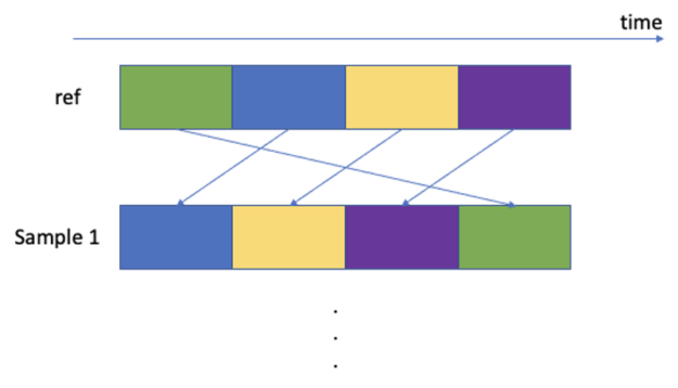
Bootstrapped datasets are used to account for the non-stationarity of time series’ future returns. A new return time series is constructed by sampling the blocks with replacement to reconstruct a time series with the same length as the original time series. Each block has a fixed length, but a random starting point in time is defined from the futures return time-series. We choose to use a block of 60 business days. This block length is motivated by a typical monthly or quarterly rebalancing frequency of dynamic rule-based strategies and by the empirical market dynamics that happen on this time scale. Papenbrock and Schwendner (2015) found multi-asset correlation patterns to change at a typical frequency of a few months.
Following is the Numba kernel to sample blocks from the reference prices matrix. Notice the `@cuda.jit` decorator, which tells Numba to just-in-time compile the boot_strap kernel.
@cuda.jit
def boot_strap(result, ref, block_size, num_positions, positions):
    sample, assets, length = result.shape
    i = cuda.threadIdx.x
    sample_id = cuda.blockIdx.x // num_positions
    position_id = cuda.blockIdx.x % num_positions
    sample_at = positions[cuda.blockIdx.x]
    for k in range(i, block_size*assets, cuda.blockDim.x):
        asset_id = k // block_size
        loc = k % block_size
        if (position_id * block_size + loc + 1 < length):
            result[sample_id, asset_id, position_id * block_size +
                   loc + 1] = ref[asset_id,  sample_at + loc]
Since stock prices are non-stationary, the stock price time series data is first converted to log returns. It serves as a reference matrix where we sample the random blocks. It is the `ref` argument in the kernel function, which has the dimension of [assets, time]. The `result` argument is the result of bootstrap sampling, which has the dimension of [sample, assets, time]. The `block_size` defines the size of the block, which is chosen for 60 business days. `num_positions` is the number of blocks that is needed to cover the whole-time length. It is calculated by:
num_positions = (length - 2) // block_size + 1`sample_positions` is an array of random times of range [0, length – block_size], which indicates the random sample starting time for the block. `sample_positions` has the size of `samples * num_positions`. For each sample, we need to sample `num_positions` of blocks to cover the whole time length, so each block can be identified by a tuple (sample_id, position_id), where position_id is in range [0, num_positions].
We mapped each GPU thread block to different sampled time blocks identified by tuple (sample_id, position_id). The following is the formula of mapping thread block id cuda.blockIdx.x to block id tuple (sample_id, position_id).
   sample_id = cuda.blockIdx.x // num_positions
   position_id = cuda.blockIdx.x % num_positions
The threads inside the thread block are used to move data elements to the result matrix. The data elements that need to be moved have two dimensions: assets and time location within a block. The following is the formula of mapping thread id to asset_id and time location.
  asset_id = k // block_size
  loc = k % block_size
To launch the Numba kernel, we can use the following Python method:
boot_strap[(number_of_blocks,), (number_of_threads,)](output,
                                                      ref,
                                                      block_size,
                                                      num_positions,
                                                      sample_positions)
Applying lessons learned to the rest of the pipeline
The rest of the computation steps follow a similar pattern as the block bootstrapping step. For example, when calculating the covariance distances, we identify that each rebalancing time period is independent of each other. So the granularity of parallelism is at the level of bootstrap scenario and rebalancing intervals. We map thread block id to sample id and rebalancing times. The threads inside thread blocks are used to move the data elements and do parallel computations (parallel CUDA sum, sort etc.). To see the details of implementation, please refer to the github repo at:https://github.com/NVIDIA/fsi-samples/tree/main/gQuant/plugins/hrp_plugin
Numba is good for accelerating algorithms in a single GPU. We can run 4096 number of scenarios in parallel in a single V100 32G GPU. However, to run 100K scenarios, it won’t fit in a single GPU. Dask is a Python library that can be used to accelerate algorithms in a cluster of GPUs. As previously shown, we already implemented a function that outputs the sampled scenarios in a GPU CuPy array similar to a NumPy array. First, we convert it to GPU DataFrame in zero-copy manner with the RAPIDS cuDF library. Dask provides a `dask.delayed` method that can annotate this function so it can be constructed into a Dask computation graph. By calling this delayed function 100k/ 4096 times, we can get the results as a dask_cudf DataFrame by the `dask.dataframe.from_delayed` method. Note, this only lazily constructs the Dask computation graph and the computation is triggered by either the ‘compute’ or ‘persist’ methods. The following steps take this dask_cudf DataFrame as input and use the `dask.map_partition` method to do the computation for each of the DataFrame partitions as if they are processing a single cudf DataFrame. Dask can smartly schedule the GPU resources to finish all the computations in parallel.
Conclusion
In this post, we described how to implement a portfolio construction algorithm with Numba/Dask. This approach provides up to 800x speed-upson the GPU, which had significant business impacts for Munich Re. We have used a similar Numba/Dask approach to accelerate a backtesting algorithm on GPU, which helped us win the STAC A3 benchmark. Hopefully, this post inspired you to take a fresh look at your existing code and start to think about how to accelerate it on GPUs.
