
Graph neural networks (GNNs) have revolutionized machine learning for graph-structured data. Unlike traditional neural networks, GNNs are good at capturing intricate relationships in graphs, powering applications from social networks to chemistry. They shine particularly in scenarios like node classification, where they predict labels for graph nodes, and link prediction, where they determine the presence of edges between nodes.
Processing large graphs in a single forward or backward pass can be computationally expensive and memory-intensive.
The workflow for large-scale GNN training typically starts with subgraph sampling to use mini-batch training. This entails feature gathering to capture needed contextual information in a subgraph. Following these, the extracted features and subgraphs are employed in neural network training. This stage is where GNNs showcase proficiency in aggregating information and enabling the iterative propagation of node knowledge.
However, dealing with large graphs poses challenges. In scenarios like social networks or personalized recommendations, graphs can have many nodes and edges, each carrying substantial feature data.
Node feature data can take up several kilobytes per vertex. As a result, the total size of node feature data can easily surpass the size of graph topology data. Sometimes reaching multiple terabytes or petabytes for the largest workloads requires large-capacity (key, value) storage.
This post introduces WholeGraph, a new feature in the RAPIDS cuGraph library. WholeGraph is a kind of graph storage, which can work together with PyG, cuGraph-PyG, DGL, cuGraph-DGL, and cuGraph-Ops to accelerate large-scale GNN training. For more information about performance and how WholeGraph addresses the challenges of inter-GPU communication bandwidth, see Optimizing Memory and Retrieval for Graph Neural Networks with WholeGraph, Part 2.
Why WholeGraph?
WholeGraph provides large-capacity and high-performance storage abstractions backed by multiple memories, such as pinned host memory and device memory. This versatility enables WholeGraph optimization performance by using the most appropriate memory type for a given task or system configuration.
WholeGraph storage can span multiple GPUs across multiple nodes. Remote memory accesses use NVIDIA NVLink P2P memory accesses or bulk transfers using NCCL.
Also, with native PyTorch support and compatibility with torch DistributedDataParallel mode, WholeGraph efficiently distributes training processes across multiple GPUs, enhancing scalability and memory optimization for large-scale graph datasets.
What WholeGraph does
WholeGraph is developed to help train large-scale GNNs. WholeGraph provides an underlying storage structure called WholeMemory. WholeMemory is a tensor-like storage. WholeMemory can efficiently organize and manipulate data in multiple dimensions, akin to tensors in deep learning frameworks.
It also provides multi-GPU support, making it optimal for NVLink systems like NVIDIA DGX A100 servers. By working with cuGraph, cuGraph-Ops, cuGraph-DGL, cuGraph-PyG, upstream DGL, and PyG, it’s easy to build GNN applications.
WholeMemory
WholeMemory can be regarded as a complete or whole view of memory on multiple GPUs. WholeMemory exposes a handle to the memory instance no matter how the underlying data is stored on multiple GPUs.
Because multiple GPUs share WholeMemory, each requires access to the entire memory space, making address mapping necessary. WholeMemory provides three address-mapping modes:
- Continuous: Offers straightforward memory access.
- Chunked: Provides a way to manage memory in distinct sections with high efficiency.
- Distributed: Enables multi-node storage but requires additional coordination for accessing data across GPUs.
Each mode has its own benefits and trade-offs, depending on the specific requirements of your application and system configuration.
Continuous
All memory from each GPU is mapped into a single continuous memory address space for each GPU. The GPU can directly access the memory using a single pointer and offset, just like using normal device memory. The software can’t tell the difference when using this mode. The hardware handles the communication required for P2P memory access.
Chunked
Memory from each GPU is mapped into different memory chunks, one for each GPU. For PyTorch, these can be a list of tensors. Here, you can still access array elements using a pointer and offset, but there are multiple pointers (one pointer per chunk). You must pick the right pointer based on the global offset and compute the new local offset value for the picked memory chunk.
Distributed
Memory from other GPUs isn’t mapped to the current GPU and direct access is not supported. You can no longer access array elements using pointers in this mode and must use WholeMemory-provided functions to access array elements. This type of WholeMemory mode can be used to create multi-node storage.
Pinned host memory
In addition to using GPU memory, WholeMemory also supports using pinned host memory. Host memory can be pinned in two ways:
- Continuous pinning: Enables multiple processes to share the same memory.
- Distributed pinning: Better suited for applications running across multiple nodes.
WholeMemory Embedding
As in large-scale GNN training, gathering node features consumes a lot of time. In some GNN applications, read and write accesses are required on node features (embedding) data when features are trainable. To help speed up feature gathering or updating learnable features, WholeGraph introduces WholeMemory Embedding for feature storage.
Compared to WholeMemory Tensor objects, WholeMemory Embedding has two more features:
- It supports caching. It can store commonly used features in a local GPU or local node in a multi-GPU or multi-node run. Alternatively, it can store features in device memory for host storage.
- It has support for sparse optimizers for trainable features. With sparse optimizers, only the affected features are updated, accelerating the training process.
WholeMemory framework integration
Although nearly all functionalities are exposed as Python objects or functions, seamless integration with deep learning (DL) frameworks can provide convenience for developers. So WholeMemory provides a DLPack capsule, which can convert WholeMemory objects into tensors for deep learning frameworks. The supported conversion method depends on the type of address-mapping modes of WholeMemory.
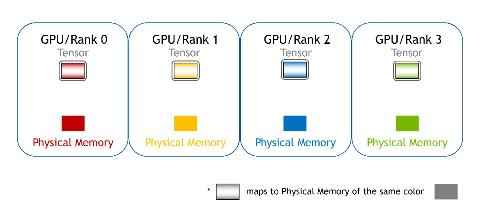
- For distributed WholeMemory, there’s no mapping to remote memory. Only local memory can be converted to a DLPack capsule and then to tensors of DL frameworks.
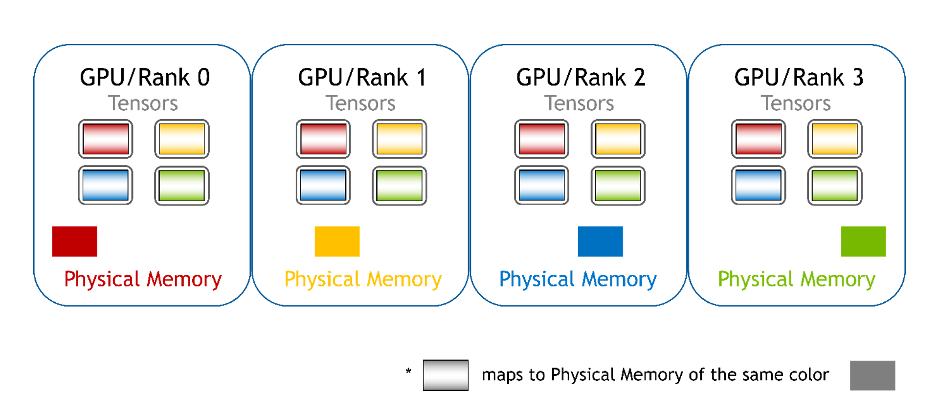
- For chunked WholeMemory, mapping to remote memory is supported. Memory chunks from all ranks can be converted to a list of DLPack capsules and imported to DL frameworks as a list of tensors.
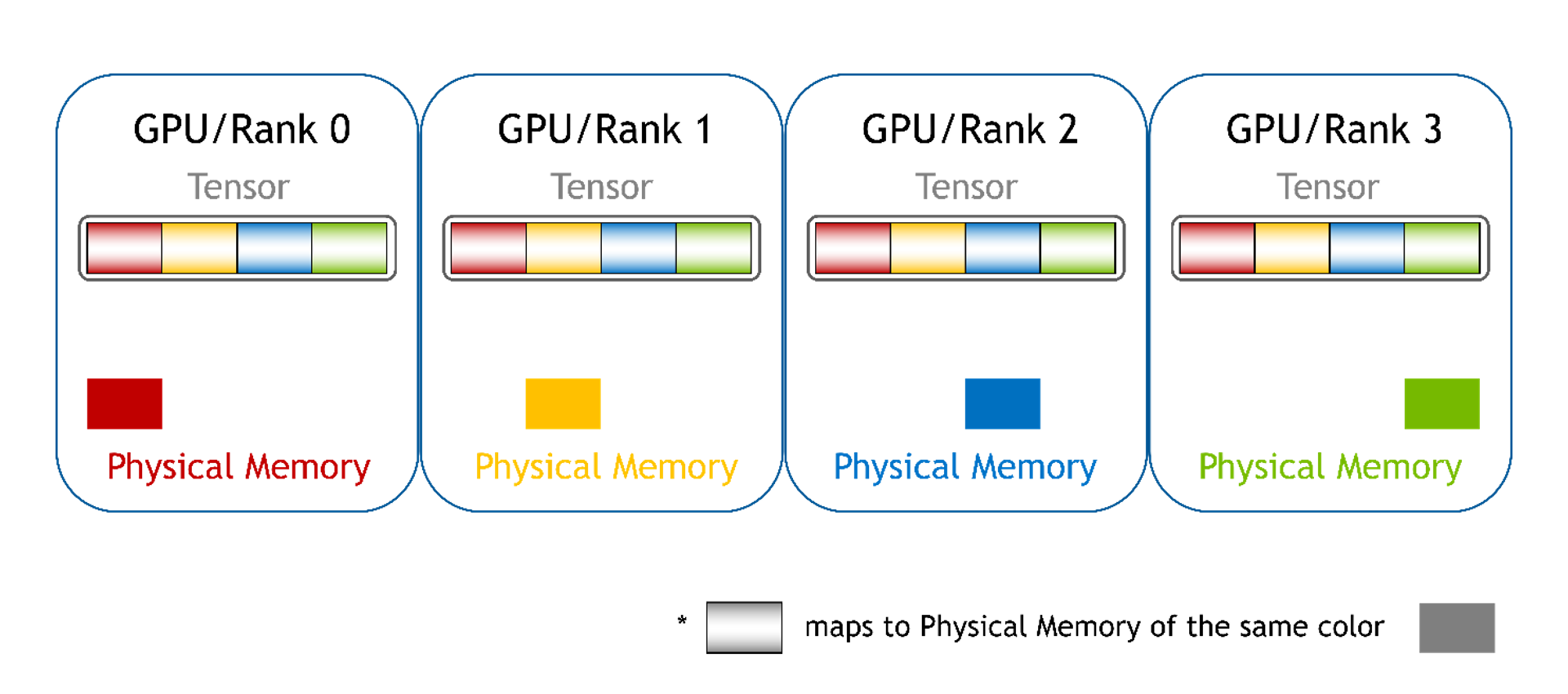
- Continuous WholeMemory has full functionality and memory is mapped into a single continuous memory address space. This can be converted into a single DLPack capsule and imported by a DL framework as a single tensor. The tensor is almost the same as other tensors from the DL framework. The difference is that its storage is on multiple GPUs. The tensor is shared by multiple processes and can be large.
Getting started
The first step is to install the WholeGraph package, which can be installed using conda or by installing from source.
To install using conda, run the following command:
> conda install -c rapidsai pylibwholegraph
To build from source, get the code from GitHub:
> git clone https://github.com/rapidsai/wholegraph.git
Next, go to the WholeGraph directory and run the build.sh script. The script is built from the source and installed in that package. Be sure to make sure that all requirements are installed per the documentation.
> cd wholegraph
> bash build.sh
Using WholeGraph
For this section on using WholeGraph, we use the ogbn-papers100M dataset as an example. The dataset is a directed citation graph of 111M papers indexed by the Microsoft Academic Graph, where each node has a 128-dim feature embedding. In this example, WholeGraph stores the feature embedding table.
To use WholeGraph, you must convert data into a binary format that WholeGraph reads. Assume that the feature embedding is in a NumPy array called feat_array, then this can be done as follows:
…
with open('feat_data.bin', 'wb') as f:
    feat_array.tofile(f)
The data is stored in a file called feat_data.bin that you can load with WholeGraph and train GNN models. The full preprocessing script for the ogbn-papers100M dataset can be found in GitHub.
Before using WholeGraph, the WholeGraph multiprocess environment must be initialized:
import pylibwholegraph.torch as wgth
wgth. init_torch_env(world_rank, world_size, local_rank, local_size)
The next step is to create a communicator that defines the set of GPU used to create WholeMemory. For example, to create a communicator of all GPUs on a local machine node, run the following command:
local_comm = get_local_node_communicator()
The two steps of initializing the WholeGraph multiprocess environment and creating a communicator can be merged into a single call. This creates the two most commonly used communicators. One is the communicator for all GPUs on a local machine node. The other is the communicator for all GPUs on all machine nodes.
global_comm, local_comm = wgth.init_torch_env_and_create_wm_comm(
    world_rank, world_size, local_rank, local_size)
After that, WholeMemory Embedding can be created to store node features. The following code example creates the embedding tables on all GPUs of the local machine node. In this example, the WholeMemory type is chunked. You don’t need a cache or sparse optimizer, so no related arguments are specified.
node_feat_wm_embedding = wgth.create_embedding_from_filelist(
    local_comm,
    "continuous",
    "cuda",
    os.path.join(node_feat_path, "node_feat.bin"),
    torch.float,
    128
With the WholeMemory Embedding created, the gather method is used to gather features. Here, indices and gathered_feature are all PyTorch tensors.
gathered_feature = node_feat_wm_embedding.gather(indices)
Besides using the WholeMemory Embedding object, you can get the WholeMemory Tensor object by calling the get_embedding_tensor method of WholeMemory Embedding:
node_feat_wm_tensor = node_feat_wm_embedding. get_embedding_tensor()
Different types of WholeMemory Tensor objects can be mapped to PyTorch tensor or tensors. For example, a continuous WholeMemory Tensor object can map to a single PyTorch tensor as follows:
node_feat_pytorch_tensor = node_feat_wm_tensor. get_global_tensor()
Here, node_feat_pytorch_tensor is a PyTorch tensor, and any PyTorch operator can use that directly while the underlying storage may be memory on multiple GPUs.
The WholeMemory Embedding table can be used for GNN training and the example is available on the /rapidsai/wholegraph GitHub repo.
Conclusion
WholeGraph offers a straightforward implementation, simplifying multi-GPU or multi-node storage setups with minimal code change. The RAPIDS team is continuously adding new features and optimizing performance in WholeGraph. For more information about performance and how WholeGraph addresses the challenges of inter-GPU communication bandwidth, see Optimizing Memory and Retrieval for Graph Neural Networks with WholeGraph, Part 2.
The code is available on the /rapidsai/wholegraph GitHub repo, where you can also submit questions and issues.
