
In this post, we detail the recently released NVIDIA Time Series Prediction Platform (TSPP), a tool designed to compare easily and experiment with arbitrary combinations of forecasting models, time-series datasets, and other configurations. The TSPP also provides functionality to explore the hyperparameter search space, run accelerated model training using distributed training and Automatic Mixed Precision (AMP), and deploy and run inference on accelerated model formats on the NVIDIA Triton Inference Server.
Accurately forecasting future time series values using previous values has proven pivotal in understanding and managing complex systems, including but not limited to power grids, supply chains, and financial markets. In these forecasting applications, single-digit percentage improvements in predictive accuracy can have vast financial, ecological, and social impacts. In addition to needing to be accurate, forecasting models also must be able to function on real-time timescale.
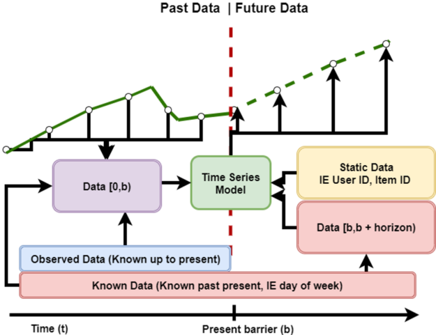
The sliding window forecasting problem, shown preceding in Figure 1, involves using prior data and knowledge of future values to predict future target values. Traditional statistical methods, such as ARIMA and its variants, or Holt-Winters Regression have long been used to perform regression for these tasks. However, as data volume has increased and the problems to solve with regression have become increasingly complex, deep learning approaches have proven their ability to represent effectively and understand these problems.
Despite the advent of deep learning forecasting models, there historically has not been a way to effectively experiment with and compare the performance and accuracy of time series models across an arbitrary set of datasets. To this end, we’re delighted to publicly open-source the NVIDIA Time Series Prediction Platform.
What is the TSPP?
The Time Series Prediction Platform is an end-to-end framework that enables users to train, tune, and deploy time series models. Its hierarchical configuration system and rich feature specification API allow for new models, datasets, optimizers, and metrics to be easily integrated and experimented with. The TSPP is designed for use with vanilla PyTorch models and is agnostic to the cloud or local platforms.
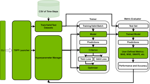
The TSPP, pictured in Figure 2, is centered around a command line-controlled launcher. Based on user input to the CLI, the launcher either instantiates a hyperparameter manager, which can run a set of training experiments in parallel or will run a single experiment by creating the described components, such as model, dataset, metric, etc.
Models supported
The TSPP supports the NVIDIA Optimized Temporal Fusion Transformer (TFT) by default. Within the TSPP, TFT training can be accelerated using multi-GPU training, automatic mixed precision, and exponential moving weight averaging. The model can be deployed using the aforementioned inference and deployment pipeline.
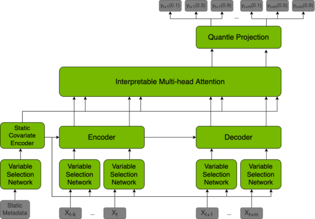
The TFT model is a hybrid architecture joining LSTM encoding and interpretable transformer attention layers. Prediction is based on three types of variables: static (constant for a given time series), known (known in advance for whole history and future), observed (known only for historical data). All of these variables come in two flavors: categorical, and continuous. In addition to historical data, we feed the model with historical values of the time series itself.
All variables are embedded in high-dimensional space by learning an embedding vector. Categorical variables embeddings are learned in the classical sense of embedding discrete values. The model learns a single vector for each continuous variable, which is then scaled by this variable’s value for further processing. The next step is to filter variables through the Variable Selection Network (VSN), which assigns weights to the inputs in accordance with their relevance to the prediction. Static variables are used as a context for variable selection of other variables and as an initial state of LSTM encoders.
After encoding, variables are passed to multi-head attention layers (decoder), which produce the final prediction. The whole architecture is interwoven with residual connections with gating mechanisms that allow the architecture to adapt to various problems.
Accelerated training
When experimenting with deep learning models, training acceleration can greatly increase the number of experimental iterations you can make in a given time. The Time Series Prediction Platform provides the ability to accelerate training with any combination of Automatic Mixed Precision, Multi-GPU Training, and Exponential Moving Weight Averaging.
Training quick start
Once one is inside the TSPP container, running the TSPP is as simple as calling the launcher with the combination of a dataset, model, and other components that you want to use. For example, to train TFT with the Electricity dataset, we simply call:
Python launch_tspp.py dataset=electricity model=tft criterion=quantile
The resulting logs, checkpoints, and initial config will be saved to outputs. For examples that include more complex workflows, please reference the repository documentation.
Automatic mixed precision
Automatic Mixed Precision (AMP) is a mode of execution for deep learning training, where applicable calculations are computed in 16-bit precision instead of 32-bit precision. AMP execution can greatly accelerate deep learning training without loss of accuracy. AMP is included in the TSPP and can be enabled by simply adding a flag to the launch call.
Multi-GPU training
Multi-GPU data parallel training provides acceleration for model training by increasing the global batch size by running model computations in parallel on all available GPUs. This approach can greatly improve model training time without loss of model accuracy, especially when many GPUs are used. It is included in the TSPP through PyTorch DistributedDataParallel and can be enabled by simply adding an element to the launch call.
Exponential moving weight averaging
Exponential Moving Weight Averaging is a technique that maintains two copies of a model, one that is being trained through backpropagation, and a second model that is the weighted average of the weights of the first model. At test and inference time, the averaged weights are used to compute outputs. This approach has proven to decrease time to convergence and increase convergence accuracy in practice, at the cost of doubling model GPU memory requirements. EMWA is included in the TSPP and can be enabled by simply adding a flag to the launch call.
Hyperparameter tuning
Model hyperparameter tuning is an essential part of the model development and experimentation process for deep learning models. For this purpose, the TSPP includes a rich integration with the Optuna hyperparameter search library. Users can run extensive hyperparameter searches by specifying hyperparameter names and distributions to search on. Once this is done, the TSPP can run multi-GPU or single-GPU trials in parallel until the desired number of hyperparameter options have been explored.
At search completion, the TSPP will return the hyperparameters of the best single run, as well as the log files of all runs. For ease of comparison, the log files are generated with the NVIDIA DLLogger and are easily searchable and compatible with Tensorboard plotting.
Configurability
Configurability in the TSPP is driven by Hydra, an open-source library provided by Facebook. Hydra allows users to define a hierarchical configuration system using YAML files that are combined at runtime, making launching runs as simple as stating ‘I want to try this model with this dataset’.
Feature specification
The feature specification, which is included in the dataset portion of configuration, is a standard description language for time-series datasets. It encodes the attributes of each tabular feature with information about whether it is known, observed, or static in the future, whether or not the feature is categorical or continuous, and many more optional attributes. This description language provides a framework for models to automatically configure themselves based on arbitrary described input.
Component integration
Adding a new dataset to the TSPP is as simple as creating a feature specification for it and describing the dataset itself. Once the feature specification and a few other key values have been defined, models integrated with the TSPP will be able to configure themselves to the new dataset.
Adding a new model to the TSPP simply requires that the model expects the data presented by the feature specification to be in the correct channel. If the model correctly interprets the feature spec, the model should work with all datasets integrated into the TSPP, past, and future.
In addition to models and datasets, the TSPP also supports the integration of arbitrary components, such as criterion, optimizers, and goal metrics. Through the use of Hydra’s direct instantiation of objects using config, users can integrate their own custom components and use them simply using the specification in a launch of the TSPP.
Inference and deployment
Inference is a key component of any Machine Learning pipeline. To this end, the TSPP has built-in support for inference that integrates seamlessly with the platform. In addition to supporting native inference, the TSPP also supports single-step deployment of converted models to NVIDIA Triton Inference Servers.
NVIDIA Triton model navigator
The TSPP provides full support for the NVIDIA Triton Model Navigator. Compatible models can be easily converted to optimized formats including TorchScript, ONNX, and NVIDIA TensorRT. In the same step, these converted models will be deployed to an NVIDIA Triton Inference Server. There is even an option to profile, analyze, and generate helm charts for a given model as part of a single step. For example, given a TFT output folder, we can convert and deploy a model to NVIDIA TensorRT format in fp16 by exporting to ONNX with the following command:
Python launch_deployment.py export=onnx convert=trt config.inference.precision=fp16 config.evaluator.checkpoint=/path/to/output/folder/
TFT Model
We benchmarked TFT within the TSPP on two datasets: the Electrical Load (Electricity) dataset from the UCI dataset repository, and the PEMs Traffic dataset (Traffic). TFT achieves strong results on both datasets, achieving the lowest seen error on both datasets and confirming the assessment of the authors of the TFT paper.
| Dataset | Mean Absolute Error | Root Mean Squared Error |
| Electricity | 43.807 | 142307.152 |
| Traffic | 0.005081 | 0.018 |
Training Performance
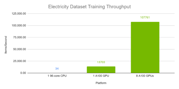
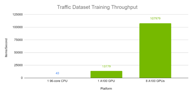
Figures 4 and 5 demonstrate the per-second throughput of TFT on the Electricity and Traffic datasets respectively. Each batch, with batch size 1024, contains a variety of time windows from different time series within the same dataset. The A100 runs were computed using Automatic Mixed Precision. As is evident, TFT has excellent performance and scaling on A100 GPUs, especially when compared with execution on a 96-core CPU.
Training time
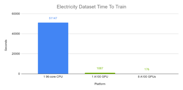
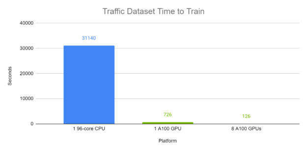
Figures 6 and 7 demonstrate the end-to-end training time of TFT on the Electricity and Traffic datasets respectively. Each batch, with batch size 1024, contains a variety of time windows from different time series within the same dataset. The A100 completed runs were computed using Automatic Mixed Precision. In these experiments, on GPU, TFT is trained in minutes, while the CPU runs trained in approximately half a day.
Inference Performance
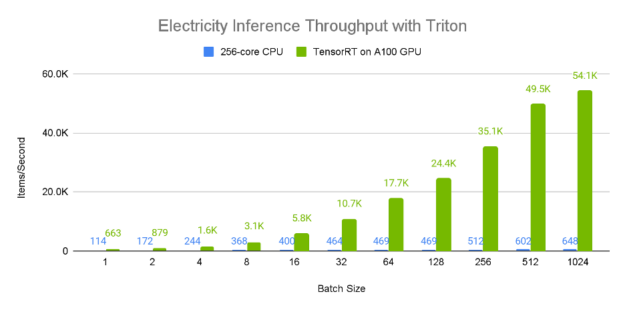
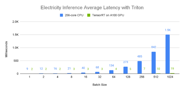
Figures 8 and 9 demonstrate the relative single-device inference throughput and average latency of an A100 80GB GPU vs a 96-core CPU across a variety of batch sizes on the electricity dataset. Since larger batch sizes generally generate greater inference throughput, we consider the 1024 element batch results, where it is apparent that the A100 GPU has incredible performance, processing approximately 50,000 samples a second. Furthermore, larger batch sizes tend to lead to higher latency as is evident from the CPU values, which seem to scale proportionally with the batch size. In contrast, the A100 GPU has a near constant average latency when compared to the CPU.
End-to-end example
Tying together the preceding examples, we demonstrate a simple training and deployment of the TFT model on the Electricity dataset. We begin by building and launching the TSPP container from the source:
cd DeeplearningExamples/Tools/PyTorch/TimeSeriesPredictionPlatform
source scripts/setup.sh
docker build -t tspp .
docker run -it --gpus all --ipc=host --network=host -v /your/datasets/:/workspace/datasets/ tspp bash
Next, we launch the TSPP with the electricity dataset, TFT, and a quantile loss. We also overload the number of epochs to train for 10. Once the model has been trained, logs, config files, and a trained checkpoint will be created in outputs/{date}/{time}, in this case, outputs/01-02-2022/:
Python launch_tspp.py dataset=electricity model=tft criterion=quantile config.trainer.num_epochs=10
Using the checkpoint directory, the model can be converted to NVIDIA TensorRT format and deployed to an NVIDIA Triton Inference Server.
Python launch_deployment.py export=onnx convert=trt config.evaluator.checkpoint=/path/to/checkpoint/folder/
Availability
The NVIDIA Time Series Prediction Platform provides end-to-end GPU acceleration from training to inference for time series models. The reference example included in the platform is optimized and certified to run on NVIDIA DGX A100 and NVIDIA-Certified Systems. For a deeper dive into the performance achieved see our Temporal Fusion Transformer benchmarks.
Organizations can start training, comparing model architectures with their own datasets, and deploying the models in production today.
