
This post is the first installment of the series of introductions to the RAPIDS ecosystem. The series explores and discusses various aspects of RAPIDS that allow its users solve ETL (Extract, Transform, Load) problems, build ML (Machine Learning) and DL (Deep Learning) models, explore expansive graphs, process geospatial, signal, and system log data, or use SQL language via BlazingSQL to process data.

RAPIDS framework was introduced in late 2018 and has since grown substantially, both, in terms of popularity as well as feature richness. Modeled after the pandas API, Data Scientists and Engineers can quickly tap into the enormous potential of parallel computing on GPUs with just a few code changes.
In this post, we will provide a gentle introduction to the RAPIDS ecosystem and showcase the most common functionality of RAPIDS cuDF, the GPU-based pandas DataFrame counterpart. We will also introduce some of the newer and more advanced capabilities of RAPIDS in later segments: NRT (near real-time) data streaming, applying BERT model to extract features from system logs, or scale to clusters of hundreds of GPU machines, among others.
cuDF is a data science building block for RAPIDS. It is an ETL workhorse allowing building data pipelines to process data and derive new features. Being part of the ecosystem, all the other parts of RAPIDS build on top of cuDF making the cuDF DataFrame the common building block. cuDF, just like any other part of RAPIDS, uses CUDA backed to power all the GPU computations. However, with an easy and familiar Python interface, users do not need to interact directly with that layer.
To help get familiar with using cuDF, we provide a handy cheat sheet that can be downloaded here: cuDF-cheat sheet.
Familiar interface for GPU processing
The core premise of RAPIDS is to provide a familiar user experience to popular data science tools so that the power of NVIDIA GPUs is easily accessible for all practitioners. Whether you’re performing ETL, building ML models, or processing graphs, if you know pandas, NumPy, scikit-learn or NetworkX, you will feel at home when using RAPIDS.
Switching from CPU to GPU Data Science stack has never been easier: with as little change as importing cuDF instead of pandas, you can harness the enormous power of NVIDIA GPUs, speeding up the workloads 10-100x (on the low end), and enjoying more productivity – all while using your favorite tools. Check the sample code below that presents how familiar cuDF API is to anyone using pandas.
import pandas as pd
import cudf
df_cpu = pd.read_csv('/data/sample.csv')
df_gpu = cudf.read_csv('/data/sample.csv')
Loading data from your favorite data sources
Reading and writing capabilities of cuDF have grown significantly since the first release of RAPIDS in October 2018. The data can be local to a machine, stored in an on-prem cluster, or in the cloud. cuDF uses fsspec library to abstract most of the file-system related tasks so you can focus on what matters the most: creating features and building your model.
Thanks to fsspec reading data from either local or cloud file system requires only providing credentials to the latter. The example below reads the same file from two different locations,
import cudf

df_local = cudf.read_csv('/data/sample.csv')
df_remote = cudf.read_csv(
    's3://<bucket>/sample.csv'
    , storage_options = {'anon': True})
cuDF supports multiple file formats: text-based formats like CSV/TSV or JSON, columnar-oriented formats like Parquet or ORC, or row-oriented formats like Avro. In terms of file system support, cuDF can read files from local file system, cloud providers like AWS S3, Google GS, or Azure Blob/Data Lake, on- or off-prem Hadoop Files Systems, and also directly from HTTP or (S)FTP web servers, Dropbox or Google Drive, or Jupyter File System.
Creating and saving DataFrames with ease
Reading files is not the only way to create cuDF DataFrames. In fact, there are at least 4 ways to do so:
From a list of values you can create DataFrame with one column,
cudf.DataFrame([1,2,3,4], columns=['foo'])Passing a dictionary if you want to create a DataFrame with multiple columns,
cudf.DataFrame({
      'foo': [1,2,3,4]
    , 'bar': ['a','b','c',None]
})
Creating an empty DataFrame and assigning to columns,
df_sample = cudf.DataFrame()
df_sample['foo'] = [1,2,3,4]
df_sample['bar'] = ['a','b','c',None]
Passing a list of tuples,
cudf.DataFrame([
      (1, 'a')
    , (2, 'b')
    , (3, 'c')
    , (4, None)
], columns=['ints', 'strings'])
You can also convert to and from other memory representations:
- From an internal GPU matrix represented as an
DeviceNDArray, - Through DLPack memory objects used to share tensors between Deep Learning frameworks and Apache Arrow format that facilitates a much more convenient way of manipulating memory objects from various programming languages,
- To converting to and from pandas DataFrames and Series.
In addition, cuDF supports saving the data stored in a DataFrame into multiple formats and file systems. In fact, cuDF can store data in all the formats it can read.
All of these capabilities make it possible to get up and running quickly no matter what your task is or where your data lives.
Extracting, transforming, and summarizing data
The fundamental data science task, and the one that all data scientists complain about, is cleaning, featurizing and getting familiar with the dataset. We spend 80% of our time doing that. Why does it take so much time? One of the reasons is because the questions we ask the dataset take too long to answer. Anyone who has tried to read and process a 2GB dataset on a CPU knows what we’re talking about. Additionally, since we’re human and we make mistakes, rerunning a pipeline might quickly turn into a full day exercise. This results in lost productivity and, likely, a coffee addiction if we take a look at the chart below.
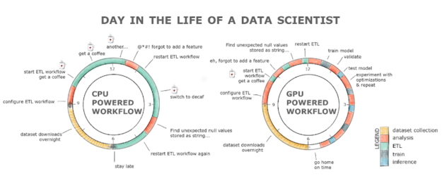
RAPIDS with the GPU powered workflow alleviates all these hurdles. The ETL stage is normally anywhere between 8-20x faster, so loading that 2GB dataset takes seconds compared to minutes on a CPU, cleaning and transforming the data is also orders of magnitude faster! All this with a familiar interface and minimal code changes.
Working with strings and dates on GPUs
No more than 3 years ago working with strings and dates on GPUs was considered almost impossible and beyond the reach of low-level programming languages like CUDA. After all, GPUs were designed to process graphics, that is, to manipulate large arrays and matrices of ints and floats, not strings or dates.
RAPIDS allows you to not only read strings into the GPU memory, but also extract features, process, and manipulate them. If you are familiar with Regex then extracting useful information from a document on a GPU is now a trivial task thanks to cuDF. For example, if you want to find and extract all the words in your document that match the [a-z]*flow pattern (like, dataflow, workflow, or flow) all you need to do is,
df['string'].str.findall('([a-z]*flow)')Extracting useful features from dates or querying the data for a specific period of time has become easier and faster thanks to RAPIDS as well.
dt_to = dt.datetime.strptime("2020-10-03", "%Y-%m-%d")
df.query('dttm <= @dt_to')
All in all, RAPIDS has changed the game when it comes to data processing, and other tasks of data scientists, not just on a local GPU box, but also at scale in data centers. Queries that used to take hours or days to process take minutes to finish, resulting in increased productivity and a lower overall cost.
Try it for yourself and download the cuDF cheatsheet!
Update 11/20/2023: RAPIDS cuDF now comes with a pandas accelerator mode that allows you to run existing pandas workflow on GPUs with up to 150x speed-up requiring zero code change while maintaining compatibility with third-party libraries. The code in this blog still functions as expected, but we recommend using the pandas accelerator mode for seamless experience. Learn more about the new release in this TechBlog post.