Optimizing End-to-End Memory Networks Using SigOpt and GPUs

Natural language systems have become the go-between for humans and AI-assisted digital services. Digital assistants, chatbots, and automated HR systems all rely on understanding language, working in the space of question answering. So what are question answering (QA) systems and why do they matter? In general, QA systems take some sort of context in the form of natural language and retrieve, summarize, or generate information based on this context. Maximizing the performance of these systems is critical if they are to be useful. QA performance is the difference between Amazon Alexa becoming a new member of the family or yet another device relegated to the back of your closet.

Research into Question Answering remains very active due to the popularity of voice-capable systems. New models and algorithms regularly out-perform each other on benchmarking tasks like the popular SQUAD challenge. Exciting areas of research include training more accurate and contextually diverse word embeddings (BERT and ELMO), evaluating variations in RNN+CNN based architectures (BiDAF, QANet), and comparing the performance of memory networks (MemN2N, Dynamic Memory Networks). Each of these approaches exemplifies practitioners using their expertise to engineer performance gains in the QA system.

Hyperparameter tuning represents a well-researched method complementary to these expert-driven approaches to further boost model performance. Although tuning typically improves performance relative to a baseline, the proportion of its improvement often differs with particular circumstances of the data, model and task. This nuance leads us to the first question for QA: where can hyperparameter tuning drive a significant improvement in performance for these expert-driven processes?

Equally important in the context of QA systems is the practicality of implementing different hyperparameter tuning methods. Each applied machine learning setting comes with different constraints in time, resources, and experts. We should consider whether these constraints point toward one method or the other for tuning. In short, if you construe performance as both accuracy and speed, will certain tuning methods be more capable for QA systems?

This post focuses on comparing the performance of memory networks and the impact of tuning on them. In particular, we focus on End-to-End Memory Networks (MemN2N) as a baseline for QA systems benchmarked on the bAbI (Babi) dataset. With MemN2N reaching an average accuracy of 86.7% and Memory Networks (MemNN) at 93.3%, MemN2N is unable to match the performance of its highly supervised counterpart (MemNN) on Babi tasks. MemN2N is an appealing baseline for QA models because of its interpretable architecture, end-to-end training, and tolerance of minimal supervision. Let’s look at how using SigOpt’s automated hyperparameter optimization product capitalizes on these qualities to impact model performance. To do so, we compare two methodologies for hyperparameter optimization:

Random Search. This is the most performant standard approach, served using SigOpt’s solution
Bayesian Optimization with Conditional Parameters: served by SigOpt and using SigOpt Conditionals, an advanced proprietary algorithmic feature.

The bAbI benchmark comprises 20 tasks. We optimize the MemN2N architecture on all 20 tasks together to offer perspective on the average performance of each tuning method for this particular benchmark. Previous work suggests Bayesian Optimization to be the most efficient and precise in finding a globally optimal hyperparameters or, in this case MemN2N architecture configuration. We use these experiments to evaluate this prediction.

To provide insight on feasibility, we provide two analyses. First, we compare CPUs to GPUs in terms of compute cost and optimization time for these tasks to serve as a benchmark for the impact of computing infrastructure on these particular systems. Second, we evaluate the trials required for random search versus Bayesian optimization to tune this architecture. Third, we compare the two methods by computing the cost per percent improvement from the MemN2N baseline. Each of these holds implications for teams facing different constraints in applied machine learning settings today.

Understanding the data

Before diving into the model architecture, let’s take a step back to understand the Babi dataset. The dataset is comprised of 20 tasks. You can see some examples in Table 1:

Table 1: Subset of examples from the full bAbI dataset. The data serves as a benchmark to ascertain the performance of a QA model.You can find the full set of tasks at https://research.fb.com/downloads/babi/.
bAbl
Task ID	Task Type	Example Data	Answer
1	Single Supporting Fact	Mary moved to the bathroom. John went to the hallway. Where is Mary?	Bathroom
3	Three Supporting Facts	Mice are afraid of wolves. Gertrude is a mouse. Cats are afraid of sheep. What is gertrude afraid of?	Wolf
4	Two Argument Relations	The hallway is east of the bathroom. The bedroom is west of the bathroom. What is the bathroom east of?	Bedroom
6	Yes/No Questions	Mary got the milk there. John moved to the bedroom. Is John in the kitchen?	No
14	Time Reasoning	Bill went back to the cinema yesterday. Julie went to the school this morning. Fred went to the park yesterday. Yesterday Julie went to the office. Where was Julie before the school?	Office
15	Basic Deduction	Mice are afraid of wolves. Gertrude is a mouse. Cats are afraid of sheep. What is gertrude afraid of?	Wolf
19	Pathfinding	The garden is west of the bathroom. The bedroom is north of the hallway. The office is south of the hallway. The bathroom is north of the bedroom. The kitchen is east of the bedroom. How do you go from the bathroom to the hallway?	S,S
20	Agent’s Motivation	Sumit is tired. Where will sumit go? Sumit went back to the bedroom. Why did sumit go to the bedroom?	Bedroom, Tired

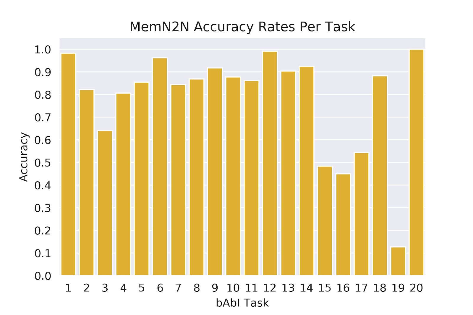
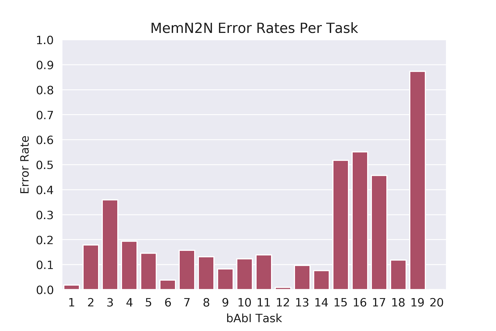
According to Facebook AI Research (FAIR), a model passing each of the 20 tasks implies it has the potential to truly understand human language and will perform well on more realistic complex data.6 (“Passing in this context means achieving 95% or greater accuracy). In other words, good performance on the Babi dataset is a “prerequisite for any system that aims to be capable of conversing with a human”. We focus on the 1k example-per-task version of the dataset. Tasks 17 and 19 perform the worst for both MemNN and MemN2N model types, with Task 17 scoring 65% accuracy for MemNN and 55% accuracy for MemN2N and Task 19 scoring 36% and 10% respectively. Along with understanding the performance of all 20 tasks, we observe the power of optimization on these lower performing tasks as well.

Model Architecture

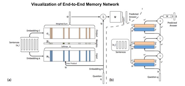
A MemN2N model has three main components: input memory representation, output memory representation, and final prediction, as shown in figure 1. These main components form a unit of the network, with the number of units (hops) itself being varied. The model training follows a pattern similar to other machine learning models. First, transform the input sentences (stories) and question to vector representations. Second, update the weights using back propogation. Finally, predict the most likely label (a singular word in the vocabulary). Through this process, embedding matrices A, B, C, and weight matrix W are updated.

End-to-end memory network diagram — Figure 1. Is a single layer of the model (b) is a three layer version. Sentences {x_i} are stories for the question answer pair transformed into input and output memory vector by embedding matrix A and C respectively. Question q is transformed in the same manner through embedding matrix B.

Sukhbaatar experiments with different variations to the base MemN2N network, including features such as positional encoding (PE), linear start (LS), random empty memories (RN), joint vs single training, and hop size. We incorporate these or similar features into our model, including PE, adding noise in gradients, joint training, and hops. We deliberately exclude LS because Bayesian optimization is typically a more efficient process to explore and exploit a search space to avoid a local minima, thereby avoiding the need for LS.3

Defining Hyperparameters

Once we define the variant of MemN2N to train, we need to define the parameters we want to optimize. Sukhbaatar trains the MemN2N model with the following parameters:

L2 norm = 40
Batch size = 32
Epochs = 60
Memory size = 50
Embedding size = 50
Learning rate = 0.01 that anneals every 15 epochs by a half until 60 epochs

As the learning strategy is critical to model performance, we choose to additionally optimize the stochastic gradient descent variant. The gradient descent variants avoid the annealing strategy, keeping model tuning consistent with current standard practices. For consistency, we compare our optimization results to a variant of Sukhbaatar’s MemN2N without annealing. Figures 2 and 3 highlight the task based accuracy for the MemN2N baseline:

MemoryN2N accuracy per task for bAbl chart — Figure 2. MemoryN2N accuracy per task for the bAbI dataset trained without annealing

Memn2n error rate per task for bAbl chart — Figure 3. MemoryN2N error rate per task for the bAbI dataset trained without annealing

We tuned gradient descent variant, word embedding size, memory size, and hop size simultaneously. We evaluated the SGD variants Adam, Adagrad, Gradient Descent with Momentum, Adadelta, and RMSprop. Ten total hyperparameters and three static parameters exist between these five SGD variants. The configuration of static parameters is as Table 2 shows:

Table 2. Static parameters used when training MemN2N
Name	Type	Value	Adam	Adagrad	Gradient Descent Momentum	Adadelta	RMSProp
Max gradient normalization	double	40	True	True	True	True	True
Batch size	double	32	True	True	True	True	True
Epochs	double	60	True	True	True	True	True

Table 3 lists all hyperparameters and which have corresponding impact in different SGD variants. In this case, True designates that the SGD variant includes the hyperparameter and False indicates that it does not:

Table 3. Hyperparameters tuned when training MemN2N and associated range values
Name	Type	Range	Adam	Adagrad	Gradient Descent Momentum	Adadelta	RMSProp
beta_1	double	[0.8, 0.99]	True	False	False	False	False
beta_2	double	[0.95, 0.9999]	True	False	False	False	False
decay_rate	double	[0.9, 0.99]	False	False	False	True	True
epsilon	double	[1e-9, 0.00001]	True	True	False	True	False
learning_rate	double	[1e-6, 1]	True	True	True	False	True
momentum_coef	double	[0.1, 0.99]	False	False	True	False	False
nesterov	categorical	True, False	False	False	True	False	False
word embedding dimension	double	[10, 100]	True	True	True	True	True
number of hops	double	[1, 3]	True	True	True	True	True
memory size	double	[1, 50]	True	True	True	True	True

SigOpt Conditionals allow for explicit relationships between the hyperparameters and the SGD variant. If a given SGD doesn’t employ a hyperparameter, it doesn’t suggest a value for that parameter. This is particularly useful when tuning deep learning architectures. For example, each layer is dependent upon the previous layer in terms of input/output and the size of the layer in a deep learning model. SigOpt Conditionals can effectively tune this layered architecture since the user explicitly defines layerwise dependencies (layer 2 depends on layer 1). SigOpt considers the parameter space to be a single contiguous space for random search, simply ignoring the hyperparameter values if they do not exist for the selected SGD.

Random search is the best of the “brute force” methods to optimization but is computationally problematic and unscalable beyond 10 hyperparameters.1,2 It relies on luck to locate a sample a point in hyperparameter space that is an optima and usually unable to find a global optima. The main difference between SigOpt Conditionals and Random search lies in SigOpt’s ability to explore and exploit the hyperparameter space.

During optimization, SigOpt learns from previously sampled points and balances sampling unsearched areas in the hyperparameter space (exploration) with homing in on the best performing region in the hyperparameter space (exploitation). The conditionals feature specifically allows explicit hyperparameter decoupling to more efficiently and effectively explore and exploit the hyperparameter space. This balance typically means that Bayesian optimization improves the accuracy of the model much faster than random search. These improvements occur more reliably for different types of models, including high dimensional models, non-continuous or irregular spaces, and circumstances that include noisy data.

Let’s examine performance in terms of compute cost and optimization speed while exploring which optimization yields the best results. We run each optimization method on AWS EC2 p2.xlarge instances using Nvidia GK210 GPUs as well as AWS EC2 c5.xlarge instances to compare GPU performance versus CPU. On demand pricing for AWS EC2 p2.xlarge at time of experiment is $0.90/hr and pricing for AWS EC2 c5.xlarge is $0.18/hr. To compare optimization methods with statistical accuracy, each optimization strategy is run 20 times on GPU. Each optimization method mentioned above require different numbers of evaluations.

Optimization Results

The following tables show the performance of each optimization method’s compute time, performance in relation to accuracy, and ROI in relation to compute cost and percent improvement. First, let’s evaluate which combination of optimization method and infrastructure type is the fastest in wall-clock time and most cost efficient. This analysis offers insight for teams facing constraints in applied settings. Table 4 summarizes results from these benchmarks.

Table 4. CPU vs GPU time and compute cost break down per evaluation. Each evaluation trains the MemN2N model for 60 epochs. Pricing: AWS EC2 p2.xlarge = $0.90/hr and EC2 c5.xlarge = $0.18/hr.
Comparing hardware-optimization method combinations for wall-clock time and computing cost considerations
Optimization Method	CPU Time per Evaluation	GPU Time per Evaluation
Random	5.43 minutes	3.30 minutes
SigOpt Conditionals	8.80 minutes	4.24 minutes

GPUs posted better results than CPUs with each optimization method. In fact, GPUs ran 1.6x to 2.1x faster than CPUs depending on the optimization method. Despite a significant increase in performance, GPU computation increases cost by 1.5-2.5x CPU cost, as c5.xlarge instances cost $0.18/hr and p2.xlarge instances cost $0.90/hr. We highly recommend using a monitoring tool to keep tabs on AWS compute time, especially if you happen to be significantly cost constrained.

Since the MemN2N architecture is similar to an RNN in terms of sequential and layer wise weighting, strategies for effective RNN training on GPUs can be applied to MemN2N.5 Using the latest versions of Tensorflow and cudNN, batch sizes that are multiples of 32 (64 for cuBLAS), large batch sizes, consolidate non-sequential matrix operations, and make layers multiples of 32 (64 for cuBLAS) all enable users to decrease GPU compute costs and train more efficiently. See Baidu’s investigation of BLAS libraries for further information on efficient computing.

Table 5 compares the optimization method, number of evaluations, average accuracy over 20 iterations, average improvement relative to MemN2N baseline, and p-values comparing the Random search variants with SigOpt Conditionals. SigOpt Conditionals outperforms Random search at 750 observations by 3x. At 15000 evaluations, Random search is still unable to match the performance of SigOpt Conditionals while costing 16x more.

Table 5: Performance breakdown across optimization methods for all 20 tasks. GPU cost =$0.90/hr used for Cost/% Improvement
All 20 Tasks
Optimization Method	Evaluations	Average Accuracy	Average Improvement (base = 78.67%)	P-value (Sigopt Conditionals vs Random Variant)	Cost per % improvement (GPU)	Best SGD Variant
Random	750	80.28%	1.61%	9.16e-08	$23.06	GradientDescentMomentum
Random	15000	82.73%	4.06%	3.30e-06	$182.88	GradientDescentMomentum
SigOpt Conditionals	750	83.51 %	4.84%	–	$9.85	GradientDescentMomentum

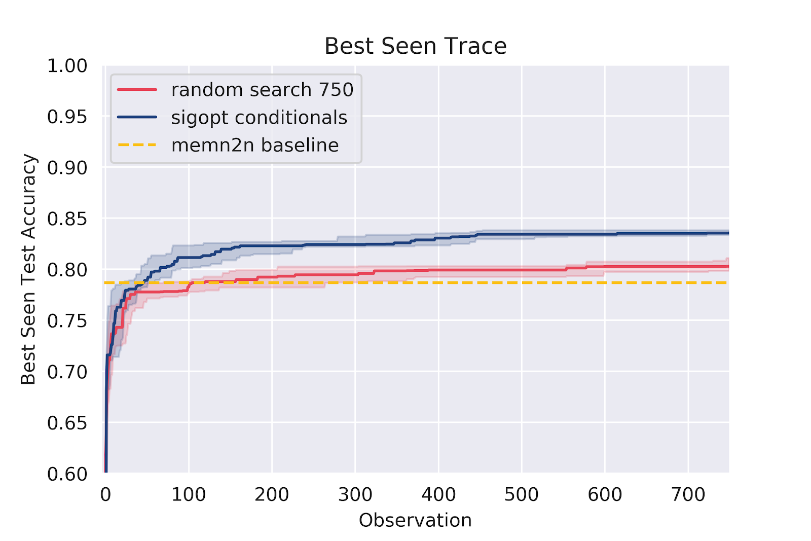
Figures 4 through 7 plots the best seen value at a given observation count. SigOpt Conditionals reaches a higher level of accuracy than Random search within a 100 observations, and Random search stagnates quickly to perform no better than the baseline.

best seen sigopt conditionals random 750 overlayed charft — Figure 4. Best seen metric at the given observation count across 20 iterations of optimization for each method. MemN2N baseline = 78.67%

best seen sigopt conditionals random zoomed 750 overlayed chart — Figure 5. Closer look at best seen metric at the given observation count across 20 iterations of optimization for each method. MemN2N baseline = 78.67%

best seen sigopt conditionals random all overlayed chart — Figure 6. Best seen metric at the given observation count across 20 iterations of optimization for each method. MemN2N baseline = 78.67%

best seen sigopt conditionals random zoomed all overlayed chart — Figure 7. Closer look at best seen metric at the given observation count across 20 iterations of optimization for each method. MemN2N baseline = 78.67%

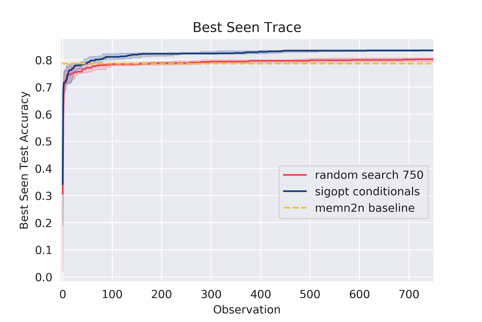
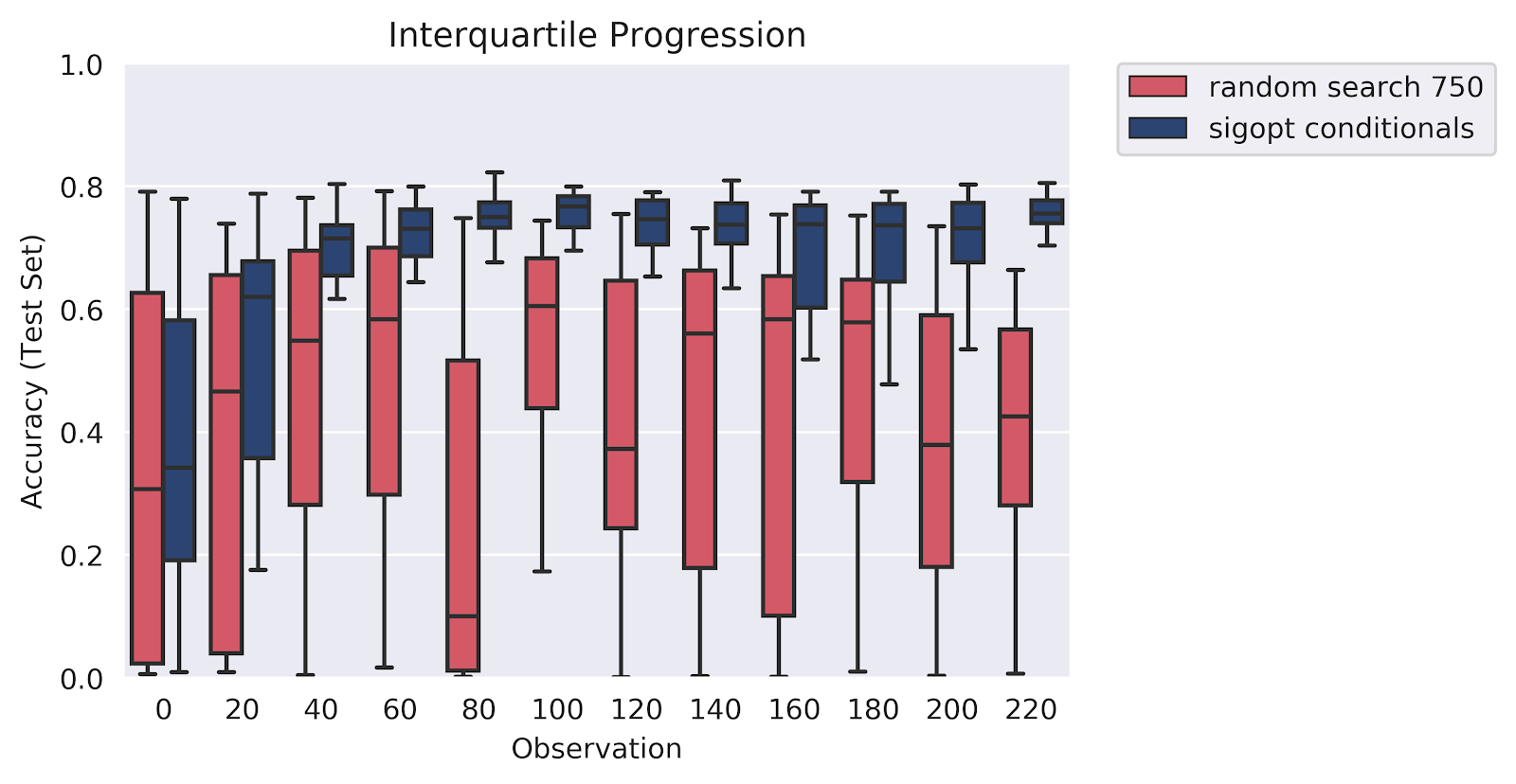
The graph in figure 8 shows howthe interquartile range is plotted along with the median behavior as observed over 20 instances for each strategy. SigOpt Conditionals outperforms Random search and identifies the optimal hyperparameter configuration well within a 100 observations, while Random search continues to naively search through the hyperparameter space.

random sigopt 750 boxplot chart — Figure 8. Interquartile progression for observed accuracy values across 20 iterations of optimization for each method

Our analysis reveals that Bayesian Optimization is clearly the most effective and efficient hyperparameter optimization method. SigOpt Conditionals locates and targets the global optima well within 80 evaluations of different hyperparameter solutions and offers a cost savings of 16x less than the Random search. SigOpt offers a substantially better approach for teams prioritizing performance, speed, or cost.

For future exploration, seeing the effects of optimization on annealing the learning rate, the effect of hyperparameter optimization on the 10k dataset, and hyperparameter tuning word embeddings could be interesting. It would also be interesting to compare the performance of an optimized MemN2N model to an optimized Dynamic Memory Network.

So what does this mean for our QA systems?

Hyperparameter optimization has a clear and positive effect on the MemN2N architecture. Apart from boosting a single model’s performance, it also allows for multiple model architectures to be tried and tested, automatically landing on a global optima. This automation leverages a practitioner’s experience by avoiding a costly hand tuning process while simultaneously empowering experimentation. Essentially, hyperparameter optimization is additive with domain expertise and goes hand-in-hand with a practitioner’s experience.

The result is that more models are put into production, and the better QA systems become. Each QA system becomes more versatile and robust after optimization. Currently, many QA, machine translation, and language modeling systems depend on the availability of massive amounts of curated data. These models could reach high levels of accuracy with minimal supervision when using hyperparameter optimization. The same systems can better understand languages such as Swahili, Hindi, and German as well as they process English speech and text using these optimizations. It is our hope that as hyperparameter optimization boosts the performance of QA systems, language processing models in general, and intelligent systems as a whole, these systems better reflect their diverse set of users and enable better human to human interaction.

What’s next?

If you’re keen on QA or NLP in general, some main conferences include ACL and EMNLP. Here’s the repo to recreate this experiment and play around with SigOpt. We’ll also be at GTC 2019 talking about Tuning the UnTunable and Orchestrate. Happy modeling!

Acknowledgements

Thanks to Harvey Cheng and Michael McCourt for their inputs and discussions.

References

1 James Bergstra, Yoshua Bengio, Random Search for Hyper-Parameter Optimization, Journal of Machine Learning Research, 13, 281-305, 2012. http://www.jmlr.org/papers/volume13/bergstra12a/bergstra12a.pdf.

2 Ian Dewancker, Michael McCourt, Scott Clark, Patrick Hayes, Alexandra Johnson, George Ke, A Stratified Analysis of Bayesian Optimization Methods, arXiv:1603.09441, 2016. https://arxiv.org/pdf/1603.09441.pdf.

3 Peter Frazier, Bayesian Optimization. Recent Advances in Optimization and Modeling of Contemporary Problems, 2018. https://pubsonline.informs.org/doi/abs/10.1287/educ.2018.0191.

4 Arvind Neelakantan, Luke Vilnis, Quoc V. Le, Ilya Sutskever, Lukasz Kaiser, Karol Kurach, James Martens, ADDING GRADIENT NOISE IMPROVES LEARNING FOR VERY DEEP NETWORKS, arXiv:1511.06807, 2016. https://arxiv.org/pdf/1511.06807.pdf.

5 Sainbayar Sukhbaatar, Arthur Szlam, Jason Weston, Rob Fergus, End to End Memory Networks, arXiv:1503.08895, 2015. https://arxiv.org/pdf/1503.08895.pdf.

6 Jason Weston, Antoine Bordes, Sumit Chopra, Alexander M. Rush, Bart van Merrienboer, Armand Joulin, Tomas Mikolov, TOWARDS AI-COMPLETE QUESTION ANSWERING : A SET OF PREREQUISITE TOY TASKS, arXiv:1502.05698, 2015. https://arxiv.org/pdf/1502.05698.pdf.

7 Jason Weston, Sumit Chopra, Antoine Bordes, Memory Networks, arXiv:1410.3916, 2014. https://arxiv.org/pdf/1410.3916.pdf.