
Recommender systems help people find what they’re looking for among an exponentially growing number of options. They are a critical component for driving user engagement on many online platforms.
With the rapid growth in scale of industry datasets, deep learning (DL) recommender models, which capitalize on large amounts of training data, have started to show advantages over traditional methods. Current DL–based models for recommender systems include the Wide and Deep model, Deep Learning Recommendation Model (DLRM), neural collaborative filtering (NCF), Variational Autoencoder (VAE) for Collaborative Filtering, and BERT4Rec among others.
There are multiple challenges when it comes to performance of large-scale recommender systems solutions: huge datasets, complex data preprocessing and feature engineering pipelines, as well as extensive repeated experimentation. To meet the computational demands for large-scale DL recommender systems training and inference, recommender-on-GPU solutions aim to provide fast feature engineering and high training throughput (to enable both fast experimentation and production retraining), as well as low latency, high-throughput inference.
In this post, we discuss our reference implementation of DLRM, which is part of the NVIDIA GPU-accelerated DL model portfolio. It covers a wide range of network architectures and applications in many different domains, including image, text and speech analysis, and recommender systems. With DLRM, we systematically tackle the challenges mentioned.
For data preprocessing tasks on massive datasets, we introduce new Spark-on-GPU tools. With automatic mixed precision training on NVIDIA Tensor Core GPUs, an optimized data loader and a custom embedding CUDA kernel, on a single Tesla V100 GPU, you can train a DLRM model on the Criteo Terabyte dataset in just 44 minutes, compared to 36.5 hours on 96-CPU threads.
We also demonstrate how to deploy trained DLRM models into production with the NVIDIA Triton Inference Server.
DLRM overview
DLRM is a DL-based model for recommendations introduced by Facebook research. Like other DL-based approaches, DLRM is designed to make use of both categorical and numerical inputs which are usually present in recommender system training data. Figure 1 shows the model architecture. To handle categorical data, embedding layers map each category to a dense representation before being fed into multilayer perceptrons (MLP). Numerical features can be fed directly into an MLP.
At the next level, second-order interactions of different features are computed explicitly by taking the dot product between all pairs of embedding vectors and processed dense features. Those pairwise interactions are fed into a top-level MLP to compute the likelihood of interaction between a user and item pair.
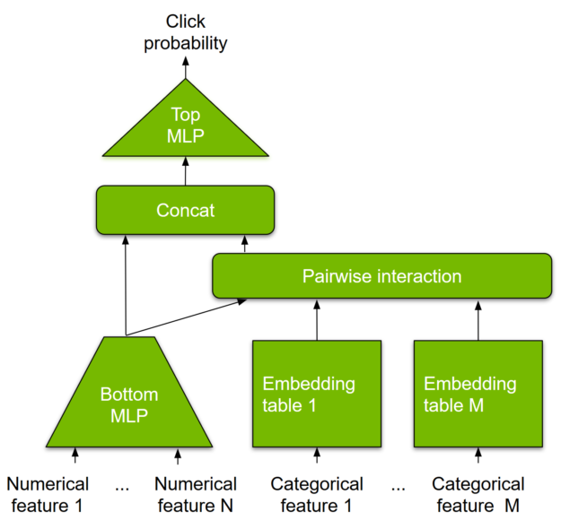
Compared to other DL-based approaches to recommendation, DLRM differs in two ways. First, it computes the feature interaction explicitly while limiting the order of interaction to pairwise interactions.
Second, DLRM treats each embedded feature vector (corresponding to categorical features) as a single unit, whereas other methods (such as Deep and Cross) treat each element in the feature vector as a new unit that should yield different cross terms. These design choices help reduce computational/memory cost while maintaining competitive accuracy.
Criteo dataset
The Criteo Terabyte click logs public dataset, one of the largest public datasets for recommendation tasks, offers a rare glimpse into the scale of real enterprise data. It contains ~1.3 TB of uncompressed click logs containing over four billion samples spanning 24 days, and can be used to train recommender system models that predict the ad clickthrough rate.
This is a large dataset in the collection of public DL datasets. Yet, real datasets can be potentially one or two orders of magnitude larger. Enterprises try to leverage as much historical data as feasible, for this generally translates into better accuracy.
For this post, we used the Criteo Terabyte dataset to demonstrate the efficiency of the GPU-optimized DLRM training pipeline. Each record in this dataset contains 40 values: a label indicating a click (value 1) or no click (value 0), 13 values for numerical features, and 26 values for categorical features. Features are anonymized and categorical values are hashed to ensure privacy.
End-to-end training pipeline
We provide an end-to-end training pipeline on the Criteo Terabyte data that help you get started with just a few simple steps.
- Clone the repository.
git clone https://github.com/NVIDIA/DeepLearningExamples
cd DeepLearningExamples/PyTorch/Recommendation/DLRM
- Build a DLRM Docker container
docker build . -t nvidia_dlrm_pyt
- Start an interactive session in the NVIDIA NGC container to run preprocessing/training and inference. The DLRM PyTorch container can be launched with:
mkdir -p data
docker run --runtime=nvidia -it --rm --ipc=host  -v ${PWD}/data:/data nvidia_dlrm_pyt bash
- Inside the Docker interactive session, download and preprocess the Criteo Terabyte dataset.
Before downloading data, you must check out and agree with the terms and conditions of the Criteo Terabyte dataset. The dataset contains 24 zipped files and require about 1 TB of disk storage for the data and another 2 TB for immediate results.
If you don’t want to experiment on the full set of 24 files, you can download a subset of files and modify the data preprocessing scripts to work on these files only.
cd preproc && ./prepare_dataset.sh && cd -
- Start training.
python -m dlrm.scripts.main --mode train --dataset /data --save_checkpoint_path model.pt
Next, we discuss several details of this training pipeline.
Data preprocessing and transformation with Spark
The original Facebook DLRM code base comes with a data preprocessing utility to preprocess the data.
- For numerical features, the data preprocessing steps include filling in missing values with 0 and normalization (shifting the values to be >=1 and taking the natural logarithm).
- For categorical features, the preprocessing transforms hashed values into a contiguous range of integers starting at 0.
This data utility, based on NumPy, runs on a single CPU thread and takes ~5.5 days to transform the whole Criteo Terabyte dataset.
We improved the data preprocessing process with Spark to make use of all available CPU threads. In the DLRM Docker image, we used Spark 2.4.5, which starts a standalone Spark cluster. This results in significant improvement in data preprocessing speed, scaling well with the number of available CPU cores. Spark outputs the transformed data in Parquet format. Finally, we converted the Parquet data files into a binary format designed especially for the Criteo dataset.
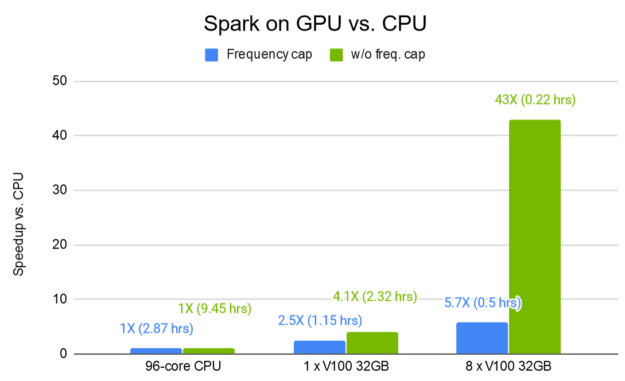
On an AWS r5d.24xl instance with 96 cores and 768 GB RAM, the whole process takes 9.45 hours (without frequency capping) and 2.87 hours (with frequency capping to map all rare categories that occur fewer than 15 times to a special category).
Spark can be improved even further. We introduced a Spark-GPU plugin for DLRM. Figure 2 shows the data preprocessing time improvement for Spark on GPU. With 8 V100 32-GB GPUs, you can further speed up the processing time by a factor of up to 43X compared to an equivalent Spark-CPU pipeline. The Spark-GPU plugin is currently in early access for select developers. We invite you to register your interest in the Spark-GPU plugin.
Our preprocessing scripts are designed for the Criteo Terabyte dataset but should work with any other dataset with the same format. The data should be split into text files. Each line of those text files should contain a single training example. An example should consist of multiple fields separated by tabulators:
- The first field is the label. Use 1 for a positive example and 0 for negative.
- The next N tokens should contain the numerical features separated by tabs.
- The next M tokens should contain the hashed categorical features separated by tabs.
You must modify data parameters, such as the number of unique values for each categorical feature and the number of numerical features in preproc/spark_data_utils.py, and Spark configuration parameters in preproc/run_spark.sh.
Data loading
We employ a binary data format, which is essentially a serialization of NumPy arrays that load particularly fast. This, combined with overlapping data loading and host2device transfer with neural net computations, allows us to achieve high GPU utilization.
Embedding tables and custom embedding kernel
DL-based recommendation models are often too large to fit onto a single device memory. This is mainly due to the sheer size of the embedding tables, which is proportional to the cardinality of categorical features and the dimensionality of the latent space (the number of rows and columns in the embedding tables).
We adopted a common practice to map all rare categorical values to a special ‘missing category’ value (here, any category that occurs fewer than 15 times in the dataset is treated as a missing category). This reduces embedding table size and avoids embedding entries that would not be sufficiently updated during training from their random initializations.
Unlike other compute-intensive layers, embedding layers are memory bandwidth–constrained. GPUs have very high bandwidth memory compared to current state-of-the-art commodity CPUs. To efficiently use the available memory bandwidth, we combine all categorical embedding tables into one single table and use a custom kernel to perform embedding lookups. The kernel uses vectorized load-store instructions for optimal performance.
Training with automatic mixed precision
Mixed precision is the use of multiple numerical precisions, such as FP32 and FP16, in a computing procedure.
Starting with the Volta architecture, NVIDIA GPUs are equipped with Tensor Cores, specialized compute units that perform matrix multiplication, a building block for linear (also known as fully connected) and convolution layers. The automatic mixed precision (AMP) features available in the NVIDIA NGC PyTorch container enables mixed precision training with minimal changes to the code base. Under the hood, AMP is provided by the NVIDIA APEX library, which enables mixed precision training by changing only three lines of your script.
In our experiments on a wide range of models and architectures in the NVIDIA DL model library, AMP usually offers speedup in the range of 1.3x up to 3x or more. For DLRM, AMP offers a 2.37x speed up compared to FP32 training. With a V100 32GB GPU, DLRM can be trained on the Criteo Terabyte dataset for one epoch in just 44 minutes, converging to an AUC value of 0.8036.
End-to-end inference pipeline
Recommender system inference involves determining an ordered list of items with which the query user most likely interacts.
For large commercial databases with millions to hundreds of millions of items to choose from (like advertisements or apps), an item retrieval procedure is usually carried out to reduce the number of items to a more manageable quantity, for example, a few hundreds to a few thousands. The methods include computationally efficient algorithms such as approximate neighborhood search or filtering based on user preferences and business rules. From there, a DL recommender model is invoked to re-rank the items. Those with the highest scores are presented to the user. This process is demonstrated in Figure 3.
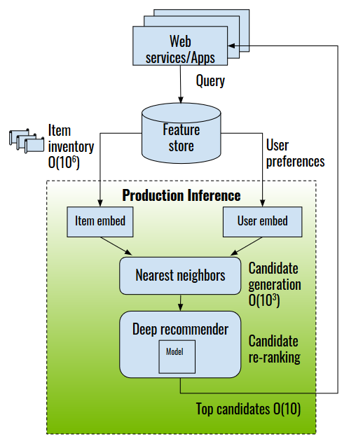
As you can see, for each query user, the number of user-item pairs to score can be as large as a few thousands. This places a heavy duty on the recommender system inference server. The server must handle high throughput to serve many users concurrently, yet operate at low latency to satisfy the stringent latency thresholds of online commerce engines.
NVIDIA Triton Inference Server provides a cloud inferencing solution optimized for NVIDIA GPUs. The server provides an inference service using an HTTP or GRPC endpoint, allowing remote clients to request inferencing for any model being managed by the server. Triton Server automatically manages and makes use of all the available GPUs.
The next section covers how to prepare the DLRM model for inference with Triton Server and see how Triton Server performs.
Prepare the model for inference
Triton Server can serve TorchScript and ONNX models, as well as others. We provides an export tool to prepare trained DLRM models ready for production inference.
Using TorchScript
Exporting pretrained PyTorch DLRM models to TorchScript models can be done using either torch.jit.script or torch.jit.trace with the following command:
python triton/deployer.py --ts-script --triton-max-batch-size 65536 --model_checkpoint dlrm.pt --save-dir /repository [other optional parameters]
This produces a production-ready model for Triton Server from a checkpoint named dlrm.pt, using the torch.jit.script and a maximum servable batch size of 65536.
Using ONNX
Similarly, an ONNX production-ready model can be created with the following command:
python triton/deployer.py --onnx --triton-max-batch-size 65536 --model_checkpoint dlrm.pt --save-dir /repository [other optional parameters]
The outcome of the export tool is a packaged directory /repository, which Triton Server can readily make use of.
Set up Triton Inference Server
With the model ready to go, Triton Server can be set up with the following steps.
- Download the Triton inference Docker image using the following command, where <tag> is the server version, for example, 20.02-py3:
docker pull nvcr.io/nvidia/tensorrtserver:<tag>
- Start the Triton Server, pointing to the exported model directory created in the previous step:
docker run --network=host -v /repository:/models nvcr.io/nvidia/tensorrtserver:<tag> trtserver --model-store=/models
Use the Triton Server perf_client tool to measure inference performance
The Triton Server comes with a handy performance client tool, perf_client. This tool stress tests the inference server with either synthetic or real data, using multiple parallel threads. It can be invoked with the following command:
/workspace/install/bin/perf_client --max-threads 10 -m dlrm-onnx-16 -x 1 -p 5000 -v -i gRPC -u localhost:8001 -b 4096 -l 5000 --concurrency-range 1 --input-data /location/for/perfdata -f result.csv
Using the perf client, we collected the latency and throughput data to populate the figures shown later in this post.
Triton Server batching strategies
By default, the exported model is deployed with the Triton Server static batching strategy: each request is immediately fulfilled. On the other hand, dynamic batching is a feature of the inference server that allows inference requests to be combined by the server, so that a batch is created dynamically. This results in the same increased throughput seen for batched inference requests.
The inferencing for a batch of inputs is performed at the same time, which is especially important for GPUs as it can greatly increase inferencing throughput. In many use cases, the individual inference requests are not batched and do not benefit from the throughput benefits of batching.
For online applications with a strict latency threshold, Triton Server is configurable so that queue time with dynamic batching is limited to an upper limit while forming the largest batch possible to maximize the throughput. In the model directory, there is a config file named config.pbtxt that can be configured with an extra batching option as follows:
ddynamic_batching {
  preferred_batch_size: [ 65536 ]
  max_queue_delay_microseconds: 7000
}
Static batch throughput
Figure 4 shows Triton Server throughput with the TorchScript DLRM model at various batch sizes. For recommender systems, large batch sizes are of the most interest. For each query user, several thousands of items are sent along in a single request for item re-ranking. Compared to an 80-thread CPU inference, a Tesla V100 32-GB GPU offers up to 20x improvement in throughput. You can see that the GPU throughput starts to saturate at around a batch size of 8K.
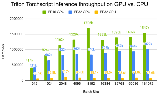
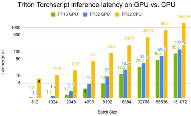
Figure 5 shows the Triton TorchScript inference latency on GPU compared to CPU. At a batch size of 8192, a V100 32-GB GPU reduces the latency by 19x compared to an 80-thread CPU inference.
Dynamic batch throughput
With dynamic batching, you can improve the throughput further over static batching. In this experiment, we set the individual per-user request batch size to 1024, and Triton maximum and preferred batch size to 65536. Figure 5 shows the latency and throughput at various request concurrency levels. Latency is broken down into client send/receive time, server queue and compute time, networking, server send/receive time.
Concurrency level is a parameter of perf_client that allows you to control the latency-throughput trade-off. By default, perf_client measures your model’s latency and throughput using the lowest possible load on the model at a request concurrency of 1. To do this, perf_client sends one inference request to the server and waits for the response. When that response is received, perf_client immediately sends another request, and then repeats this process.
At higher concurrency levels of N, perf_client immediately fires up requests one after another without waiting for the previous request to be fulfilled, while maintaining at any time at most N outstanding requests.
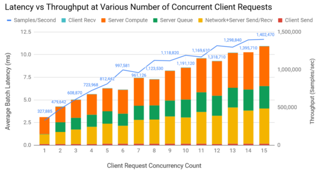
Figure 6 shows that if you have a 10-ms upper bound on latency, you can achieve a throughput of 1,318,710 samples/sec. This means ~1288 users can be served per second, each within the 10-ms latency limit, on a single V100 GPU, assuming that you want to score 1024 items for each user and that the user requests come at a uniform rate of maximum 12 requests within any 10-ms window.
Conclusion
In this post, we walked through a complete DLRM pipeline, from data preparation to training to production inference. The GPU-optimized DLRM is available from the NVIDIA deep learning model zoo, under /PyTorch/Recommendation/DLRM. We provide ready-to-go Docker images for training and inference, data downloading and preprocessing tools, and Jupyter demo notebooks to get you up and running quickly. Trained models can then be prepared for production inference in one simple step with our exporter tool. We also invite you to register your interest for early access to the Spark-GPU component.
DLRM forms part of NVIDIA Merlin, a framework for building high-performance, DL–based recommender systems. To learn more about Merlin and the larger ecosystem, see the recent post, Announcing NVIDIA Merlin: An Application Framework for Deep Recommender Systems.
We cordially invite you to try out and benefit from our newly developed tools for your recommender system applications. Your issues and feature requests help guide future development. We are excited to see what you can do with this model on your own data.
