Optimizing Data Transfer Using Lossless Compression with NVIDIA nvcomp

One of the most interesting applications of compression is optimizing communications in GPU applications. GPUs are getting faster every year. For some apps, transfer rates for getting data in or out of the GPU can’t keep up with the increase in GPU memory bandwidth or computational power. Often, the bottleneck is the interconnect between GPUs or between CPU and GPU.

Things became more balanced with the introduction of DGX systems and NVLink, but the interconnect bandwidth remains the bottleneck for most workloads running in the cloud over many nodes connected with Ethernet or InfiniBand. In such systems, the ingress and egress bandwidth per GPU is usually on the same order of magnitude as PCIe. Lossless data compression helps to reduce the off-chip traffic and can directly result in application performance gains, as long as you can achieve fast compress and decompress rates on the GPU.

There have been many research papers on GPU compression algorithms and implementations but no library has existed, until now. In this post, we introduce NVIDIA nvcomp, a new core NVIDIA library with API actions for the efficient compression and decompression of data on the GPU. This library provides easy-to-use methods to compress and decompress buffers on the GPU using various parallel compression methods.

Example of a communication-limited application

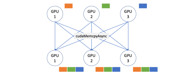
A diagram showing three GPUs performing an AllGather operation. — *Figure 1*. *All-gather communication pattern.*

To showcase the benefits of nvcomp, here’s a simple all-gather micro-benchmark. The all-gather pattern (Figure 1) is a common pattern in applications that require duplicating data across many devices or GPUs. Imagine loading a large dataset into K GPUs’ memories, from CPU memory (K=3 in Figure 1). The naive way would be to copy the whole dataset K times over PCIe, so that every GPU has a copy.

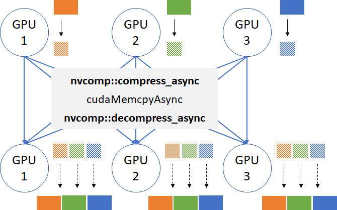
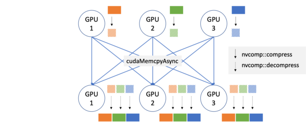
A better approach is to split the dataset into K pieces (orange, green, and blue in Figure 1), and send one piece to each GPU, and then let them gather the remaining K-1 pieces without using the CPU. When the GPU interconnect is slow (PCIe, Ethernet, or InfiniBand), fast compression and decompression on the GPU lets you send less data over the wires and improve the performance. Figure 2 shows what the application would look like with GPU compression enabled.

A diagram showing three GPUs compressing their respective chunks of a dataset, performing an AllGather operation, and then decompressing the chunks of the dataset. — *Figure 2*. *All-gather communication pattern with compression.*

For the testing platform, we selected an AWS g4dn.12xlarge instance with 4x T4s connected over PCIe. There are a couple of reasons for choosing this platform:

GPU-to-GPU bandwidth is PCIe limited.
We can stay within one node and don’t need to introduce APIs for multi-node communications.

Even though we’re showing an example application running on a single node, the same communication bottleneck would show up in many multi-node applications, and GPU compression can be easily applied in the same way.

Here is the baseline code for all-gather within one node:

for(int i = 0; i < gpus; ++i) {
  for(int j = 0; j < gpus; ++j) {
    cudaMemcpyAsync(dest_ptrs[j][i], dev_ptrs[i], chunk_bytes[i],
                    cudaMemcpyDeviceToDevice, streams[j][i]);
  }
}
for(int i = 0; i < gpus; ++i) {
  for(int j = 0; j < gpus; ++j) {
    cudaStreamSynchronize(streams[i][j]);
  }
}

For the dataset, we used Fannie Mae’s Single-Family Loan Performance Data, also available for download at RAPIDS Mortgage Data. It is a real dataset that represents the credit performance of Fannie Mae mortgage loans. This dataset is used to train models to perform home loan risk assessment. For more information, see RAPIDS Accelerates Data Science End-to-End.

For our tests, we picked one of the largest quarters, 2009Q2, which consists of 4.2 GB of data in raw-text format (CSV), and benchmarked compression on various columns separately. We chose a diverse set of columns with different data types and numbers of valid entries. All other columns from the dataset are similar to at least one of the selected columns.

Figure 3 shows the all-gather performance results for no-compressed (baseline), and two compression methods available currently in nvcomp, LZ4 and cascaded. The effective throughput is computed as the total uncompressed size of the data produced by the all-gather operation (the column size, B, multiplied by the number of GPUs, K, minus one) divided by the total time to perform the operation, including compression, $T_{compression}$ ; decompression, $T_{decompression}$ ; and any required data transfer, $T_{transfer}$ .

$\mathrm{Effective Throughput} =\dfrac{B*(K-1)}{T_{compression} + T_{transfer} + T_{decompression}}$

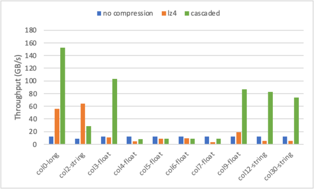
A chart showing the throughput of performing an AllGather operation using no compression, LZ4 compression, and Cascaded compression. On six of the ten datasets, LZ4 and Cascaded output perform no-compression by a large factor. — *Figure 3*. *Effective* *all-gather system throughput using different compression methods on four NVIDIA T4s connected via PCIe on an AWS g4dn.12xlarge instance.*

There are three types of columns: integer, float, and string. The cascaded scheme supports integer input only, so 32-bit floating-point numbers and string-byte streams were interpreted as 32-bit integers in this case. Here, we used one run-length encoding (RLE) stage, one delta stage, and bit-packing for the cascaded method. Later in this post, we explain the algorithm and all the stages in detail.

You can see that by using nvcomp, you can achieve up to 150 GB/s all-gather throughput on column 0, which translates into a 12x end-to-end speed-up compared to the baseline no-compression case bottlenecked by PCIe rates. Cascaded compression demonstrates the best result on columns 0, 3, 9, 12, and 30, achieving >75 GB/s throughput, while LZ4 outperforms cascaded on one of the string columns (2) reaching more than 60 GB/s.

Cascaded compression performs best on integer columns or columns with repeated values due to RLE and delta working on sequences up to 8 bytes long. Columns with longer strings, such as column 2, may have repeated sequences that cannot be effectively compressed by RLE. However, LZ4 considers a large window of previous entries and can compress these repeated sequences. Some floating-point columns (4, 5, 6, 7) with few repeats don’t compress well with either scheme, as current nvcomp compression schemes do not consider the special floating-point structure. As a result, on these columns, you see a slowdown from using compression due to the additional time it takes to run compression and decompression in addition to the transfer.

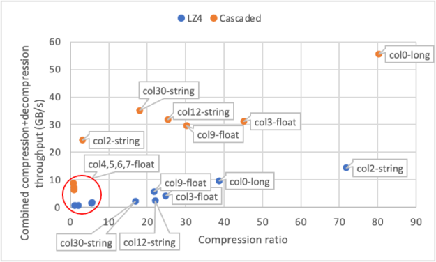
Figure 4 shows a scatter plot of combined compression+decompression throughput (Y axis) and compression ratios (X axis) for all the benchmarked columns. Each point represents one column’s result using either cascaded (orange) or LZ4 (blue) methods. The throughput is computed as the number of bytes used by the column divided by the total time it takes to perform compression and decompression. For both schemes, you see a clear correlation between compression ratio and throughput. Columns with a low compression ratio (4, 5, 6, 7) achieve low throughput, while columns with a high compression ratio typically have higher throughput as well. This is because highly compressible columns require less work and fewer memory accesses to compress and decompress.

*Figure 4.* *Compression ratio and throughput for the columns.*

In addition to the AWS instance with T4s, we also tested the same benchmark on a four-GPU quad from a DGX-1. In such a system, each GPU has 125 GB/s total egress bandwidth to peer GPUs. On some columns, nvcomp compression improves all-gather bandwidth by 2-4x even for this tightly connected system!

We’ve demonstrated the all-gather micro-benchmark results here, but there are many other communication patterns that would benefit from compression. One notable example is all-to-all that’s present in any MapReduce computations, or when moving from model parallelism to data parallelism in DL applications (for example, in recommender systems like DLRM with very large embedding tables). This post doesn’t cover those use cases in detail, but you’re welcome to experiment with your dataset, provide feedback, and request new features on the nvcomp GitHub issues page.

Now that you’ve seen the performance gains, let us show you how easy it is to integrate and use nvcomp in your applications.

Optimizing data transfer with nvcomp

Here’s how the all-gather micro-benchmark is modified to use compression algorithms from nvcomp. For simplicity, assume that each GPU sends exactly one chunk to each remote GPU.

To compress data on the GPU, you must first create a Compressor object for each GPU. In this case, you are using LZ4Compressor.

LZ4Compressor<T>** compressors = new LZ4Compressor<T>*[gpus];
for(int gpu=0; gpu < gpus; ++gpu) {
  cudaSetDevice(gpu);
  compressors[gpu] = new LZ4Compressor<T>(dev_ptrs[gpu], chunk_sizes[gpu], 1 << 16);
}

After this is done, you must get the required amount of temporary GPU space to perform the compression and allocate it. Here, you allocate one temporary buffer per stream.

for(int gpu=0; gpu < gpus; ++gpu) {
  cudaSetDevice(gpu);
  temp_bytes[gpu] = compressors[gpu]->get_temp_size();
   // Use one temp buffer for each stream on each gpu
   for(int j=0; j<gpus; ++j)
     cudaMalloc(&d_temp[gpu][j], temp_bytes[gpu]));
}

Next, you must get the required size of the output location and allocate it. For this, nvcomp provides the function get_max_output_size to compute the maximum output size for a given compressor. The maximum size is often larger than the actual size of compressed data. This is because the exact size of the output is not known until compression has run. The method get_max_output_size is not required to be called, as long as the size of the provided buffer for compressed data is safely within the limits required by the compressor.

for(int gpu=0; gpu < gpus; ++gpu) {
  cudaSetDevice(gpu);
  comp_out_bytes[gpu] = compressors[gpu]->get_max_output_size(
d_temp[gpu][0], temp_bytes[gpu]);
  cudaMalloc(&d_comp_out[gpu], comp_out_bytes[gpu]));
}

Then, allocate the numGPU memory buffers on each GPU to store the decompressed data.

for(int gpu=0; gpu < gpus; ++gpu) {
  d_decomp_out.push_back(new T*[gpus]);
  cudaSetDevice(gpu);
  for(int chunkId=0; chunkId<gpus; ++chunkId)
    cudaMalloc(&d_decomp_out[gpu][chunkId], chunk_sizes[chunkId]*sizeof(T));
}

After you have the temporary and all output memory allocations created, you can launch the compression tasks:

for(int gpu=0; gpu<gpus; ++gpu) {
  cudaSetDevice(gpu);
  compressors[gpu]->compress_async(d_temp[gpu][0], temp_bytes[gpu],
d_comp_out[gpu], &comp_out_bytes[gpu], streams[gpu][0]);
}
// Synchronize to make sure the sizes of the compressed buffers are written to CPU
for(int gpu=0; gpu<gpus; ++gpu)
  cudaStreamSynchronize(streams[gpu][0]);

The compression function is asynchronous with respect to the GPU and follows the stream semantics. Because you don’t know the exact size of the compressed data before the kernel is completed, you must synchronize the streams before issuing memory copies to the peer GPUs. You can avoid this synchronization and pipeline the kernels with memory copies if the latter is implemented as GPU kernels. We leave this exercise for you to try out in the benchmark code.

After you finish compression, you can send the compressed buffers over to remote GPUs. The data is copied from d_comp_out[i] to dest_ptrs[j][i] for all i = 0..gpus-1 and j = 0..gpus-1. The code for memory copies is identical to the all-gather baseline listing shown earlier, except you’re sending the compressed data.

Then, you create decompressor objects, one per communication pair. The Decompressor class understands the format by reading the metadata stored in the compressed stream, so this code can be reused for any compressor, LZ4 or cascaded.

Decompressor<T>** decompressors = new Decompressor<T>*[gpus*gpus];
for(int gpu=0; gpu < gpus; ++gpu) {
  cudaSetDevice(gpu);
  // Create decompressors for each chunk on each gpu
  for(int chunkIdx=0; chunkIdx<gpus; ++chunkIdx) {
    idx = gpu*chunks+chunkIdx;
    if (chunkIdx != gpu)
      decompressors[idx] = new Decompressor<T>(dest_ptrs[gpu][chunkIdx],
comp_out_bytes[chunkIdx], streams[gpu][chunkIdx]);
  }
}

Finally, you issue decompression kernels:

for(int gpu=0; gpu < gpus; ++gpu) {
  cudaSetDevice(gpu);
  for(int chunkIdx=0; chunkIdx < gpus; ++chunkIdx) {
    if (chunkIdx != gpu) {
      idx = gpu*chunks+chunkIdx;
      decompressors[idx]->decompress_async(d_temp[gpu][chunkIdx],
temp_bytes[gpu], d_decomp_out[gpu][chunkIdx], decomp_out_bytes[idx],
streams[gpu][chunkIdx]);
    }
  }
}

For more information about the full benchmark code, see benchmarks/benchmark_allgather.cpp. The benchmark also supports sending multiple chunks for each pair of GPUs. you may notice a slight performance improvement by increasing the number of chunks for some cases. Feel free to experiment with the provided code!

LZ4: Generic compressor for arbitrary data

LZ4 is a byte-oriented compression scheme focused on simplicity and speed. It encodes that data as a series of literals and matches. Each token is composed of a series of literals and the location and length of matches of previously compressed data to copy to the output stream. The minimum length of a match is four, as any match shorter would result in a token that takes up the same amount or more space than the uncompressed data. As a result, when LZ4 is used on incompressible data, it only expands it by at most 1/255. This makes LZ4 well-suited for compressing arbitrary data. Figure 5 shows the layout of a compressed token.

A diagram showing the five different components of an LZ4 compression token, the header, the literal LSIC, the literals, the offset, and the match LSIC. — *Figure 5. The structure of an LZ4 compression token, and how it is expanded to the uncompressed stream*.

Header: The header byte contains two 4-bit numbers. The first is the number of literals in the token, representing a range of 0–15. The second is the number of matches in the token minus four, representing a range of 4–19.
Literal linear small-integer codes: If the number of literals in the token is 15 or greater, then there are a series of LISCs to represent the larger number of literals. If the number of literals in the token is less than 15, this is omitted.
Literals: The raw literals to be copied to the output stream upon decompression.
Offset: The offset going backwards, from the last literal written to the output stream. The value can be 0-65535.
Match LSIC: If the number of matches in the token is 19 or greater, then there are another series of LSICs representing the larger number of matches. If the number of matches in token is less than 19, this is omitted.

To parallelize LZ4 effectively on the GPU, you break up datasets into blocks and compress each block concurrently by a thread block on the GPU, for both compression and decompression. You also use a single warp per thread block, to ensure that you can use warp-level primitives to coordinate threads.

During compression, each of the 32 threads in the warp reads a byte from the uncompressed input stream and compares with the other threads for potential matches. The threads also use a hash table to look for potential matches earlier in the stream. Using warp-level primitives, the match that results in the fewest literals being written is selected (greedy matching). At this point, the threads cooperatively write the compressed token to the output stream.

To parallelize decompression, you use a shared memory buffer to read the compressed input stream from global memory with all threads. You then parallelize the copy of literals across threads in the warp, as well as the copy of matches.

We have also implemented a “batched” C API for LZ4 for use in all-to-all, scatter, and gather-like operations. This API allows multiple independent memory locations to be compressed and decompressed concurrently and independently.

Cascaded: Fast and efficient compressor for integer analytics data

If you have some knowledge of the dataset, you can use specific compression methods that provide even better compression ratios with less work than general schemes like LZ4. For example, if you have a dataset of integers with many repeated elements, you can scan the data one time and store the number of repeated instances of each value, also known as RLE. nvcomp cascaded compression uses a series of these simple compression methods to quickly compress data that contains common patterns and structure.

Because cascaded compression uses a series of simple compression algorithms, it is more amenable to parallelization and can achieve high compression and decompression throughput on modern GPUs. To show this, consider column 0 from the mortgage dataset (all-gather benchmark performance shown in Figure 3). Column 0 contains a series of 64-bit integers with many duplicates, in ascending order. This type of data is well-suited to the different methods used by the cascaded compression scheme. The cascaded compression scheme uses the following simple compression techniques as building blocks:

RLE—Scans the dataset and encodes each set of repeated values with two numbers: the value and length of the run (number of repetitions). For example, 1,1,1,1,5,5 would be encoded as vals:(1,5), runs:(4,2). We use primitives from the CUB library to efficiently perform this on GPUs.
Delta encoding–Replaces each element in a sequence with the difference between it and the previous value. For example, 5,7,5,2,2 would be encoded as 5,2,-2,-3,0. This method does not directly compress many sequences but is effective in conjunction with the other building blocks.
Bit-packing–A bit-level operation that aims to reduce the number of bits required to store each value. It stores a base value and encodes each element as an offset from that base. For example, 5,6,9,5 encodes as 5:0,1,4,0. This allows each element to be stored using fewer bits.

Using the RLE, delta, and bit-packing building blocks, you can assemble various cascaded schemes. Figure 6 shows how to connect multiple building blocks to form a cascaded compression scheme.

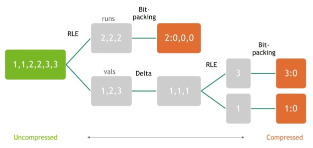
A diagram showing an example of a multi-stage Cascaded compression scheme. RLE, delta, and bitpacking layers are chained together to form the overall cascaded compression on the input dataset. — *Figure 6. Multiple stages of cascaded compression: RLE->Delta->RLE->bit-packing.*

Figure 6 shows that the RLE and delta layers are interleaved, and a final bit-packing is performed on all resulting runs and values. The number of RLE and delta layers is configurable and can have a big impact on the compression ratio of a given dataset. To get the best performance using cascaded compression, it is helpful to select the best configuration for each input dataset. To accomplish this, we are working on an auto-selector that analyzes a given dataset and quickly determines the best cascaded compression configuration to use. This auto-selector will be available with a new version of nvcomp in an upcoming release.

Choosing the best compression scheme: Cascaded vs. LZ4

While the simplicity of cascaded compression provides high throughput, it is not well-suited for many types of inputs, including strings or datasets that are not highly structured. For example, column 2 of the mortgage dataset used in the all-gather benchmark above contains various strings. This dataset has many repeated characters, so it is highly compressible using LZ4, which achieves a compression ratio of 71.8. Cascaded compression, however, only provides a compression ratio of 3.2. For general compression of arbitrary data, LZ4 is typically better suited, and cascaded compression should be reserved for numerical and analytical datasets.

On suitable numerical data, cascaded compression can provide higher throughput and compression than LZ4. On column 0 of the mortgage dataset, which is ideal for cascaded compression, it provides a compression ratio of 80, nearly twice that of LZ4. It also achieves nearly 4x the combined compression and decompression throughput of LZ4, at 56 GB/s for a T4.

Get started with nvcomp

In this post, we introduced a new NVIDIA library that lets you easily optimize your GPU data transfers by using efficient parallel compression algorithms, such as LZ4 and cascaded methods. The library is still in its infancy and we’re actively working on new features and more efficient compression methods. Here are some of the things we’re working on:

More compression methods, including GPU-friendly entropy encoding and LZ variants
Auto-selector for cascaded compression to choose the best RLE/Delta/bp setting
Performance improvements for LZ4 and batched API for cascaded compression
Integration with other CUDA libraries and frameworks

Go explore the nvcomp library on GitHub: https://github.com/NVIDIA/nvcomp — it’s fully open source. Try out our compressors in your applications and file feature requests, or simply study our GPU implementations. Maybe they’ll inspire you to build your own compression schemes. Share your ideas and contribute!