
Data Scientists deal with algorithms daily. However, the data science discipline as a whole has developed into a role that does not involve implementation of sophisticated algorithms. Nonetheless, practitioners can still benefit from building an understanding and repertoire of algorithms.
In this article, the sorting algorithm merge sort is introduced, explained, evaluated, and implemented. The aim of this post is to provide you with robust background information on the merge sort algorithm, which acts as foundational knowledge for more complicated algorithms.
Although merge sort is not considered to be complex, understanding this algorithm will help you recognize what factors to consider when choosing the most efficient algorithm to perform data-related tasks. Created in 1945, John Von Neumann developed the merge sort algorithm using the divide-and-conquer approach.
Divide and conquer
To understand the merge sort algorithm, you must be familiar with the divide and conquer paradigm, alongside the programming concept of recursion. Recursion within the computer science domain is when a method defined to solve a problem involves an invocation of itself within its implementation body.
In other words, the function calls itself repeatedly.
Divide and conquer algorithms (which merge sort is a type of) employ recursion within its approach to solve specific problems. Divide and conquer algorithms decompose complex problems into smaller sub-parts, where a defined solution is applied recursively to each sub-part. Each sub-part is then solved separately, and the solutions are recombined to solve the original problem.
The divide-and-conquer approach to algorithm design combines three primary elements:
- Decomposition of the larger problem into smaller subproblems. (Divide)
- Recursive utilization of functions to solve each of the smaller subproblems. (Conquer)
- The final solution is a composition of the solution to the smaller subproblems of the larger problem. (Combine)
Other algorithms use the divide-and-conquer paradigm, such as Quicksort, Binary Search, and Strassen’s algorithm.
Merge sort
In the context of sorting elements in a list and in ascending order, the merge sort method divides the list into halves, then iterates through the new halves, continually dividing them down further to their smaller parts.
Subsequently, a comparison of smaller halves is conducted, and the results are combined together to form the final sorted list.
Steps and implementation
Implementation of the merge sort algorithm is a three-step procedure. Divide, conquer, and combine.
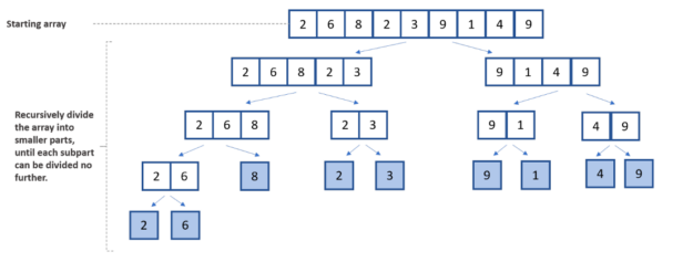
The divide component of the divide-and-conquer approach is the first step. This initial step separates the overall list into two smaller halves. Then, the lists are broken down further until they can no longer be divided, leaving only one element item in each halved list.
The recursive loop in merge sort’s second phase is concerned with the list’s elements being sorted in a particular order. For this scenario, the initial array is sorted in ascending order.
In the following illustration, you can see the division, comparison, and combination steps involved in the merge sort algorithm.

To implement this yourself:
- Create a function called merge_sort that accepts a list of integers as its argument. All following instructions presented are within this function.
- Start by dividing the list into halves. Record the initial length of the list.
- Check that the recorded length is equal to 1. If the condition evaluates to true, return the list as this means that there is just one element within the list. Therefore, there is no requirement to divide the list.
- Obtain the midpoint for a list with a number of elements greater than 1. When using the Python language, the // performs division with no remainder. It rounds the division result to the nearest whole number. This is also known as floor division.
- Using the midpoint as a reference point, split the list into two halves. This is the divide aspect of the divide-and-conquer algorithm paradigm.
- Recursion is leveraged at this step to facilitate the division of lists into halved components. The variables ‘left_half’ and ‘right_half’ are assigned to the invocation of the ‘merge_sort’ function, accepting the two halves of the initial list as parameters.
- The ‘merge_sort’ function returns the invocation of a function that merges two lists to return one combined, sorted list.
def merge_sort(list: [int]):
    list_length = len(list)

    if list_length == 1:
        return list

    mid_point = list_length // 2

    left_half = merge_sort(list[:mid_point])
    right_half = merge_sort(list[mid_point:])

return merge(left_half, right_half)- Create a ‘merge’ function that accepts two lists of integers as its arguments. This function contains the conquer and combine aspects of the divide-and-conquer algorithm paradigm. All following steps are executed within the body of this function.
- Assign an empty list to the variable ‘output’ that holds the sorted integers.
- The pointers ‘i’ and ‘j’ are used to index the left and right lists, respectively.
- Within the while loop, there is a comparison between the elements of both the left and right lists. After each comparison, the output list is populated within the two compared elements. The pointer of the list of the appended element is incremented.
- The remaining elements to be added to the sorted list are elements obtained from the current pointer value to the end of the respective list.
def merge(left, right):
    output = []
    i = j = 0

    while (i < len(left) and j < len(right)):
        if left[i] < right[j]:
            output.append(left[i])
            i +=1
        else:
            output.append(right[j])
            j +=1
    output.extend(left[i:])
    output.extend(right[j:])

    return output

unsorted_list = [2, 4, 1, 5, 7, 2, 6, 1, 1, 6, 4, 10, 33, 5, 7, 23]
sorted_list = merge_sort(unsorted_list)
print(unsorted_list)
print(sorted_list)
Performance and complexity
Big O notation is a standard for defining and organizing the performance of algorithms in terms of their space requirement and execution time.
Merge sort algorithm time complexity is the same for its best, worst, and average scenarios. For a list of size n, the expected number of steps, minimum number of steps, and maximum number of steps for the merge sort algorithm to complete, are all the same.
As noted earlier in this article, the merge sort algorithm is a three-step process: divide, conquer, and combine. The ‘divide’ step involves the computation of the midpoint of the list, which, regardless of the list size, takes a single operational step. Therefore the notation for this operation is denoted as O(1).
The ‘conquer’ step involves dividing and recursively solving subarrays–the notation log n denotes this. The ‘combine’ step consists of combining the results into a final list; this operation execution time is dependent on the list size and denoted as O(n).
The merge sort notation for its average, best, and worst time complexity is log n * n * O(1). In Big O notation, low-order terms and constants are negligible, meaning the final notation for the merge sort algorithm is O(n log n). For a detailed analysis of the merge sort algorithm, refer to this article.
Evaluation
Merge sort performs well when sorting large lists, but its operation time is slower than other sorting solutions when used on smaller lists. Another disadvantage of merge sort is that it will execute the operational steps even if the initial list is already sorted. In the use case of sorting linked lists, merge sort is one of the fastest sorting algorithms to use. Merge sort can be used in file sorting within external storage systems, such as hard drives.
Key takeaways
This article describes the merge sort technique by breaking it down in terms of its constituent operations and step-by-step processes.
Merge sort algorithm is commonly used and the intuition and implementation behind the algorithm is rather straightforward in comparison to other sorting algorithms. This article includes the implementation step of the merge sort algorithm in Python.
You should also know that the time complexity of the merge sort method’s execution time in different situations, remains the same for best, worst, and average scenarios. It is recommended that merge sort algorithm is applied in the following scenarios:
- When dealing with larger sets of data, use the merge sort algorithm. Merge sort performs poorly on small arrays when compared to other sorting algorithms.
- Elements within a linked list have a reference to the next element within the list. This means that within the merge sort algorithm operation, the pointers are modifiable, making the comparison and insertion of elements have a constant time and space complexity.
- Have some form of certainty that the array is unsorted. Merge sort will execute its operations even on sorted arrays, a waste of computing resources.
- Use merge sort when there is a consideration for the stability of data. Stable sorting involves maintaining the order of identical values within an array. When compared with the unsorted data input, the order of identical values throughout an array in a stable sort is kept in the same position in the sorted output.
