Kaggle is an online community that allows data scientists and machine learning engineers to find and publish data sets, learn, explore, build models, and collaborate with their peers. Members also enter competitions to solve data science challenges. Kaggle members earn the following medals for their achievements: Novice, Contributor, Expert, Master, and Grandmaster. The quality and quantity of work produced in competitions, notebooks, datasets, and discussions dictate each member’s level in the community.
This post gives a high-level overview of the winning solution in the Kaggle IEEE CIS Fraud Detection competition. We discuss the steps involved and some tips from Kaggle Grandmaster, Chris Deotte, on what his winning team did that made a difference in the outcome. We go over domain knowledge, exploratory data analysis, feature preprocessing and extraction, the algorithms used, model training, feature selection, hyperparameter optimization, and validation.
Fraud detection Kaggle challenge

In this challenge, IEEE partnered with the world’s leading payment service company, Vesta Corporation, in seeking the best solutions for fraud prevention. Successful ML models improve the efficacy of fraudulent transaction alerts, helping hundreds of thousands of businesses reduce fraud loss and increase revenue. This competition required participants to benchmark machine learning models on a challenging, large-scale dataset from Vesta’s real-world e-commerce transactions. The competition ran between July to October 2019, attracting 126K submissions from 6,381 teams with over 7.4K competitors from 104 countries.
NVIDIA was represented in this competition by four members of the Kaggle Grandmasters of NVIDIA (KGMON) team, in three different leading teams. Chris Deotte (cdeotte) from the USA was part of the first-place team, Gilberto Titericz (Giba) from Brazil and Jean-Francois Puget (CPMP) from France were part of the second-place team, and Christof Henkel (Dieter) from Germany was part of the 6th place team.
Kaggle process
Kaggle competitions work by asking users or teams to provide solutions to well-defined problems. Competitors download the training and test files, train models on the labeled training file, generate predictions on the test file, and then upload a prediction file as a submission on Kaggle. After you submit your solution, you get a ranking on the public leaderboard and a private leaderboard, which is only visible at the end of the competition. At the end of the competition, the top three scores on the private leaderboard obtain prize money.
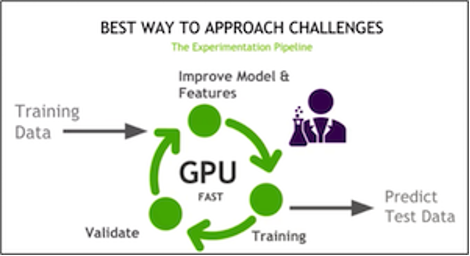
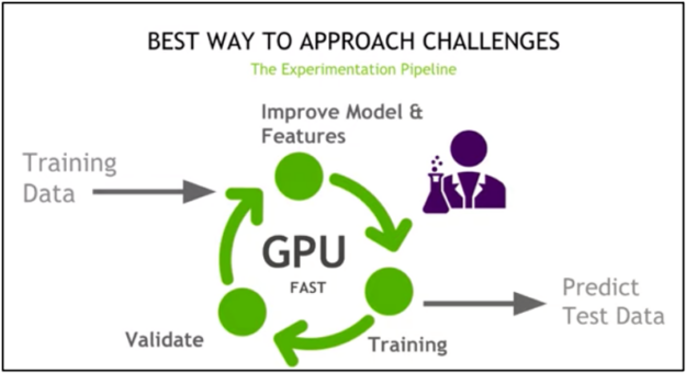
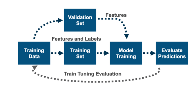
A general competition tip is to set up a fast experimentation pipeline on GPUs, where you train, improve the features and model, and then validate repeatedly.
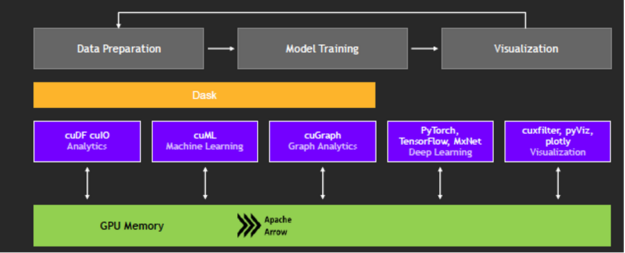
With the RAPIDS suite of open-source software libraries and APIs, you can execute end-to-end data science and analytics pipelines entirely on GPUs. RAPIDS relies on NVIDIA CUDA primitives for low-level compute optimization but exposes GPU parallelism and high memory bandwidth through user-friendly Python interfaces. The RAPIDS DataFrame library mimics the pandas API and is built on Apache Arrow to maximize interoperability and performance.
Focusing on common data preparation tasks for analytics and data science, RAPIDS offers a familiar DataFrame API that integrates with Scikit-Learn and various machine learning algorithms without paying typical serialization costs. This allows acceleration for end-to-end pipelines, from data prep and machine learning to deep learning.
Fraud detection domain knowledge
In this competition, the goal was to predict the probability that an online credit card transaction is fraudulent, as denoted by the target label isFraud. A crucial part of data science is finding the interesting properties in the data with domain knowledge. First, we give a brief overview of credit card fraud detection.
This competition is an example of supervised machine learning classification. Supervised machine learning uses algorithms to train a model to find patterns in a dataset with target labels and features. It then uses the trained model to predict the target labels on a new dataset’s features.
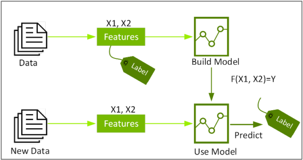
Classification identifies the class or category to which an item belongs, based on the training data of labels and features. Features are the interesting properties in the data that you can use to make predictions. To build a classifier model, you extract and test to find the features of interest that most contribute to the classification. For feature engineering for credit card fraud, the goal is to distinguish normal card usage from fraudulent unusual card usage, for example, features that measure the differences between recent and historical activities.
For online credit card transactions, there are features associated with the transaction or credit card holder and features that can be engineered from transaction histories.
Features associated with the transaction:
- Date and time
- Transaction amount
- Merchant
- Product
Features associated with the credit card holder:
- Card type
- Credit card number
- Expiration date
- Billing address (street address, state, zip code),
- Phone number
- Email address
Possible features generated from transaction history:
- Number of transactions a credit card holder has made in the last 24 hours (holder features plus device ID and IP address)
- Same or different credit card numbers?
- Same or different shipping addresses?
- The total amount a credit cardholder has spent in the last 24 hours
- Average amount last 24 hours compared to the historical daily average amount
- Number of transactions made from the same device or IP address in the last 24 hours
- Multiple online charges in close temporal proximity?
- Frequent fraud at a specific merchant?
- Group of fraud charges in certain areas?
- Multiple charges from a merchant within a short time span?
Vesta data set
The test and training data consisted of two files each, which can be joined by TransactionID: identity and transaction. The transaction file contained features associated with the online transaction and features engineered by Vesta.
TransactionDT: Timedelta from a given reference datetime (not an actual timestamp).TransactionAMT: Transaction payment amount in USD.ProductCD: Product code, the product for each transaction.card1–card6: Payment card information, such as card type, card category, issue bank, country, and so on.addr: Address.dist: Distance.P__emaildomainandR__emaildomain: Purchaser and recipient email domains.C1–C14: Counting, such as how many addresses are associated with the payment card, and so on. The actual meaning is masked.D1–D15: Timedelta, such as days between previous transactions, and so on.M1–M9: Match, such as names on card and address, and so on.Vxxx: Vesta-engineered rich features, including ranking, counting, and other entity relations.
Figure 5 shows a preview of part of the transaction data.


The identity file contains identity information: network connection information (IP, ISP, Proxy, and so on) and a digital signature (UA, browser, OS, version, and so on) associated with the credit card transactions.
The field names are masked:
DeviceTypeDeviceInfoid_12–id_38
Exploratory data analysis
Exploratory data analysis (EDA) is performed before, during, and after feature engineering to understand the data set better. The EDA for this competition was difficult, with 450 columns and masked names and meanings. The winning team did a detailed EDA, and we review just part of it here.
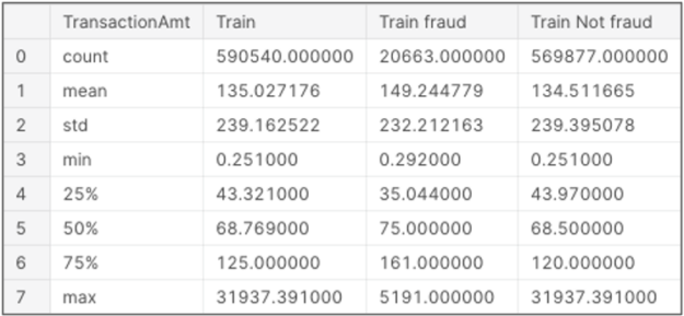
EDA uses data visualization, statistics, and queries to find important variables, interesting relations among the variables, anomalies, patterns, and insights. You can examine how the data is distributed using summary statistics with the pandas describe function. This function gives count, mean, std, min, max, and lower, 50, and upper percentiles for numeric types and count, unique, most common, and frequency of the most common strings. The following table shows summary statistics for the transaction amount, a critical feature in fraud:
A value count on the target label shows that only 3.5% of the transactions are labeled fraudulent. Typically, fraudulent transactions make up a small percentage of transactions.
| isFraud | Count | Percent |
| 0 | 569877 | 0.965 |
| 1 | 20663 | 0.034 |
Correlation can help you understand the linear relationship between features and between features and the target. A correlation can range between -1 (perfect negative relationship) and +1 (perfect positive relationship), with 0 indicating no straight-line relationship.
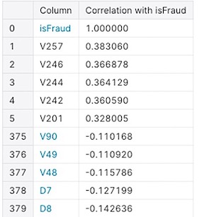
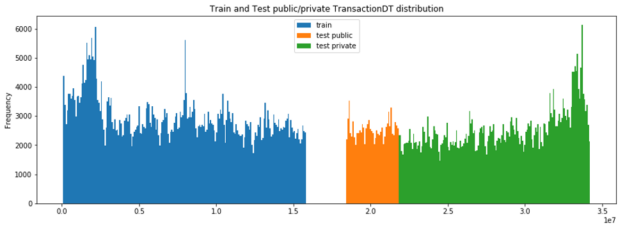
Visualizing the data helps with feature selection by revealing trends in the data. Histograms or bar charts help visualize the distribution of a feature. For example, TransactionDT (timedelta) compared to the transaction frequency in the following chart (Figure 8) shows a time gap between the training and test data.
Scatterplots visualize the relationship between two features (correlation, ratio, difference). The following scatterplot shows the transaction amount values over time (TransactionDT).

Chris’s EDA of the 340 V and Id columns determined many missing values (NAN), and that the column values were redundant and correlated. Columns were removed with the following process:
- Groups of V columns were searched to find those that shared a similar NAN structure.
- For each block of V columns with a similar NAN structure, the correlation was used to find correlated (r > 0.75) groups within that block.
- Within the correlated group, the column with the most unique values was kept (because it contained the most information), and all the other V columns from that group were removed.
- Afterward, these reduced groups were further evaluated using feature selection.
Feature preprocessing: Categorical features
Categorical features represent types of data divided into categories. For example, there are two card types: credit and debit. Categorical features that have a meaningful order—for example, unsatisfactory, satisfactory, and excellent—are called ordinal categorical features. To be used in most machine learning algorithms, nonnumeric features must be transformed into numbers representing each feature’s value. This is called different things by different frameworks: ordinal, categorical, string encoding, indexing, or factorizing. The pandas factorize method can be used to obtain a distinct numeric representation of an array of strings when all that matters is identifying different values. The factorizing method also reduces memory and turns NAN (missing values) into a number (such as -1). The Scikit-Learn OrdinalEncoder converts an array of features to ordinal integers.
Feature generation
Feature engineering and feature selection is an iterative process that starts with engineering new features, training a model, and then testing the model predictions against the target labels. The goal is to determine which features improve the model’s prediction accuracy. You repeat this process, along with hyperparameter tuning, until you are satisfied with the model’s accuracy.
Feature generation creates new features using knowledge about the problem and data. In the real-world example, you saw that fraud features could be derived from the transaction history. In this dataset, some features have already been derived:
C1–C14: Counting.D1–D15: Timedelta.M1–M9: Match.Vxxx: Vesta-engineered rich features.
Here are some ways that feature columns can be analyzed, combined, and transformed to create new features:
- Splitting or combining columns
- Encoding target, frequency, and aggregation
Splitting or combining columns
If this correlates better with the target, combine columns or split one column into two.
- For the tree-based algorithms to be able to split on these features, Chris split
TransactionAmt“1230.45” intoDollars“1230” andCents“45”. - Chris combined columns
card1,addr1, andP_emaildomain, to create a new feature because the interaction of these features combined correlated better with the target.
Encoding target, frequency, and aggregation
To detect credit card fraud, you are looking for unusual credit card behavior. Target, frequency, and aggregation encodings add features that measure the rarity of features or combinations of features.
With target encoding, features are replaced or added with the probability of the categorical value corresponding to the target. For example, if 3% of fraudulent transactions are of card type “debit,” then the value “debit” is replaced with .03.
With frequency encoding, features are replaced or added with the count of the categorical value. For example, to add a column for how frequently a card region (card1) occurs in transactions, you can add a value count column for that feature, as in the following code example:
temp = df['card1'].value_counts().to_dict()
df['card1_counts'] = df['card1'].map(temp)
Chris used frequency encoding to create the following new features:
addr1_FEcard1_FEcard2_FEcard3_FEP_emaildomain_FEcard1_addr1_FEcard1_addr1_P_emaildomain_FE
Aggregation encoding adds features based on feature aggregation statistics, such as mean or standard deviation for groups of features. This allows machine learning algorithms such as decision trees to determine if a value is common or rare for a particular group. Some of the essential features in this competition were new columns created from group aggregations of other columns.
You can calculate group statistics by providing pandas with three variables: group, variable of interest, and type of statistic. For example, the following code example adds to each row the average TransactionAmt value for that row’s card1 group, allowing the ML algorithm to determine if a row has an abnormal TransactionAmt value for the card1 value (the card holder’s region).
temp = df.groupby('card1')['TransactionAmt'].agg(['mean'])
    .rename({'mean':'TransactionAmt_card1_mean'},axis=1)
df = pd.merge(df,temp,on='card1',how='left')
Chris used feature aggregation statistics to create the following new features:
●	TransactionAmt_card1_mean, TransactionAmt_card1_std
●	TransactionAmt_card1_addr1_mean, TransactionAmt_card1_addr1_std
●	TransactionAmt_card1_addr1_P_emaildomain_mean
●	TransactionAmt_card1_addr1_P_emaildomain_std, D9_card1_mean, D9_card1_std
●	D9_card1_addr1_mean, D9_card1_addr1_std
●	D9_card1_addr1_P_emaildomain_mean, D9_card1_addr1_P_emaildomain_std
●	D11_card1_mean, D11_card1_std, D11_card1_addr1_mean, D11_card1_addr1_std
●	D11_card1_addr1_P_emaildomain_mean, D11_card1_addr1_P_emaildomain_std
ML algorithms used by the winning team
Chris used XGBoost as part of the first-place solution, and his model was ensembled with team member Konstantin’s CatBoost and LGBM models.
It is vital to get an understanding of XGBoost, CatBoost, and LGBM to first grasp the algorithms upon which they’re built: decision trees, ensemble learning, and gradient boosting.
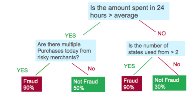
Decision trees create a model that predicts the target label by evaluating a tree of if-then-else and true/false feature questions and estimating the minimum number of questions needed to assess the probability of making a correct decision. Decision trees can be used for classification to predict a category or regression to predict a continuous numeric value.
Gradient boosting decision trees (GBDTs) are a decision tree ensemble learning algorithm similar to random forest for classification and regression. Ensemble learning algorithms combine multiple ML models to obtain a better model. Both random forest and GBDT build a model consisting of multiple decision trees; the difference is how they are built and combined.
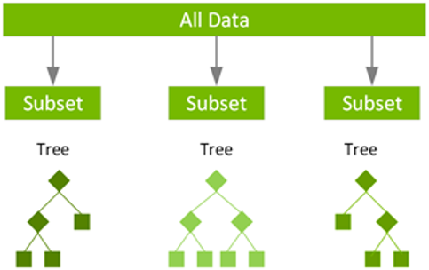
Random forest uses a technique called bagging to build full decision trees in parallel from random bootstrap samples of the data set and features. The final prediction is an average of all the decision tree predictions.
GBDT uses a technique called boosting to iteratively train an ensemble of shallow decision trees with each iteration using the residual error of the previous model to fit the next model. The final prediction is a weighted sum of all the tree predictions. Random forest bagging minimizes the variance and overfitting, while GBDT boosting reduces the bias and underfitting.
XGBoost (eXtreme Gradient Boosting) is a leading, scalable, distributed variation of GBDT. With XGBoost, trees are built in parallel instead of sequentially. XGBoost follows a level-wise strategy, scanning across gradient values and using these partial sums to evaluate the quality of splits at every possible split in the training set.
The NVIDIA RAPIDS team works closely with the DMLC XGBoost organization, and GPU-accelerated XGBoost now includes seamless, drop-in GPU acceleration, which significantly speeds up model training and improves accuracy.
LightGBM is an open-source, gradient boosting framework from Microsoft. Like XGBoost, it is fast and efficiently builds trees in parallel. A major difference is that it builds trees leaf-wise instead of row by row. CatBoost is a newer open-source gradient boosting on decision trees library developed by Yandex.
Evaluating the model
To evaluate the model’s accuracy, you must test the model’s predictions against the target labels. To do this, split the training file that has labeled data, train the model on part of the data, and test the predictions with the rest. There are various methods for splitting and training validation. When dealing with time series or time-related data, you should use time-based splitting rather than random splitting. Because this data set is time-related, make sure that you train on data that is earlier in time than the validation data.
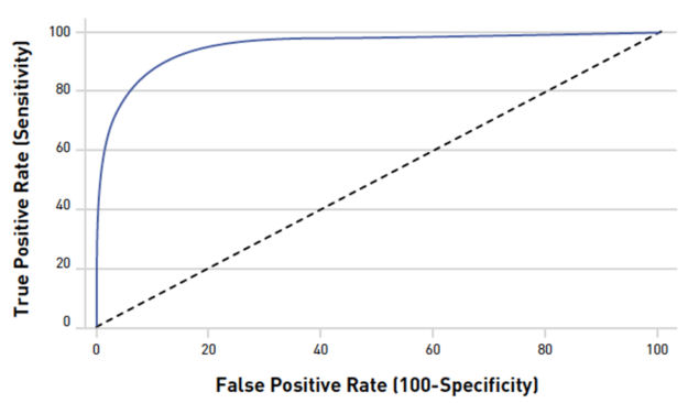
For this competition, the submissions were evaluated on AUC (Area Under the ROC Curve). Therefore, you’d want to use this measurement when evaluating your model’s predictions during training. AUC measures the ability of the model to classify true positives from false positives correctly. A random predictor would have .5 (the diagonal dashed line). The closer the value is to 1, the better its predictions are.
Hyperparameter tuning
Hyperparameter optimization tunes the model’s properties that can be set for training to find the most accurate possible model; for example, the depth of a decision tree.
To maximize the power of XGBoost to find the most accurate possible model, it’s critical to select the optimal hyperparameters. The choice of optimal hyperparameters is between underfitting and overfitting a model—where the model predictions match how the data behaves and is also generalized enough to predict on unseen data.
XGBoost has many parameters to tune and most of the parameters about bias variance tradeoff. Here is an explanation of a few:
n_estimators: The number of trees in the model. Increasing this number improves accuracy and increases training time. You can have a high number of estimators and not risk overfitting with early stopping. For more information about early stopping, see later in this post.max_depth: Maximum depth of a tree. Too shallow underfits; too deep overfits.learning rate(eta): The number to use for reducing the tree weights for boosting. Decreasing prevents overfitting but requires more trees and training time for accuracy.
Chris used the following hyperparameters for his winning model:
clf = xgb.XGBClassifier(
            n_estimators=5000,
            max_depth=12,
            learning_rate=0.02,
            subsample=0.8,
            colsample_bytree=0.4,
            missing=-1,
            eval_metric='auc',
            tree_method='gpu_hist'
        )
The XGBoost fit method can train the model on a training set, track and report the performance on a test set with the specified validation metric and stop after the specified number of early stopping rounds if the validation metric does not improve. In this example from Chris’s notebook, the model trains on the training set, evaluates on eval_set, stops after 100 rounds if the AUC metric does not improve, and prints out the results.
    h = clf.fit(X_train.loc[idxT,cols], y_train[idxT],
        eval_set=[(X_train.loc[idxV,cols],y_train[idxV])],
        verbose=50, early_stopping_rounds=100)
Feature selection
After feature engineering, you must select only the features that are most important for the model accuracy. Too many features can cause overfitting and poor performance.
After feature engineering, Chris had 242 features. For feature selection, he built 242 models. Each model was trained using one feature on the first month (calculated using TransactionDT) of the training data, and then predictions were tested on the last month of the training data. If training AUC and validation AUC was not above 0.5, then the feature was removed. This removed 19 features.
The remaining features were evaluated by training on the first 75% of the data and testing the predictions with the last 25%. The result with the XGBoost model with 216 features achieved AUC = 0.9363. The XGBoost model automatically calculates feature importance, which can be retrieved from the model and used to better understand the features and feature selection. Figure 14 shows the feature importance values for Chris’s XGBoost model after feature selection and training.

New features from aggregation encoding
After extensive EDA, Chris’s team created a credit card client unique ID, UID, from the card1, addr1, and D1 features:
X_train['day'] = X_train.TransactionDT / (24*60*60)
X_train['UID'] = X_train.card1_addr1.astype(str)+'_'+np.floor(X_train.day-X_train.D1).astype(str)

X_test['day'] = X_test.TransactionDT / (24*60*60)
X_test['UID'] = X_test.card1_addr1.astype(str)+'_'+np.floor(X_test.day-X_test.D1).astype(str)
The UID value was used to create more features from feature aggregation statistics to further determine if credit card behavior was rare or common for these credit card identifying features.
The following features were created from the UID:
UID_FE, TransactionAmt_UID_mean, TransactionAmt_UID_std, D4_UID_mean, D4_UID_std, D9_UID_mean, D9_UID_std, D10_UID_mean, D10_UID_std, D15_UID_mean, D15_UID_std, C1_UID_mean, C2_UID_mean, C4_UID_mean, C5_UID_mean, C6_UID_mean, C7_UID_mean, C8_UID_mean, C9_UID_mean, C10_UID_mean, C11_UID_mean, C12_UID_mean, C13_UID_mean, C14_UID_mean, M1_UID_mean, M2_UID_mean, M3_UID_mean, M4_UID_mean, M5_UID_mean, M6_UID_mean, M7_UID_mean, M8_UID_mean, M9_UID_mean, UID_P_emaildomain_ct, UID_dist1_ct, UID_DT_M_ct, UID_id_02_ct, UID_cents_ct, C14_UID_std, UID_C13_ct, UID_V314_ct, UID_V127_ct, UID_V136_ct, UID_V309_ct, UID_V307_ct, UID_V320_ct
The UID column itself was not used in training to avoid overfitting. For more information, see the resources mentioned in the Conclusion section.
Chris’ local validation with the new UID-aggregated features included achieved AUC = 0.9472. In Figure 15, seven of the UID-engineered features are now included in the most important.

Final model training and predictions submission
The final step, which can be repeated, is to submit a prediction file to the Kaggle competition. The test file consists of public and private parts. Predictions are scored and ranked on the public leaderboard for the public part and the private leaderboard for the private part. The private leaderboard is revealed when the competition is finished.
A sample submission for this competition should be in the following format: For each TransactionID value in the test.csv file, you must predict a probability for the isFraud variable.
TransactionID,isFraud
3663549,0.5
3663550,0.5
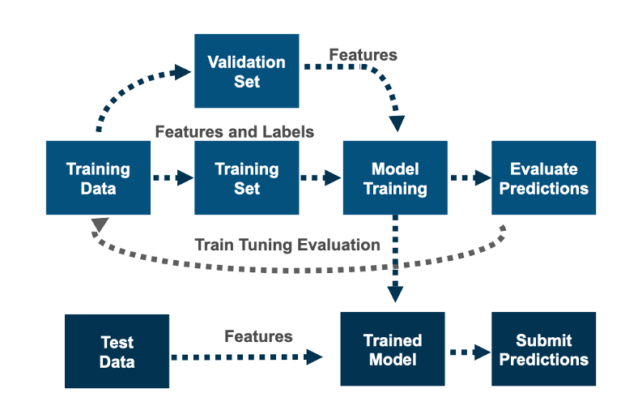
After training, tuning, and feature selection, you retrain the model on the training data before predicting on the test file. Chris’s model was trained on the training file to predict on the test file using GroupKFold training validation data splitting, with ordered months as non-overlapping groups. This makes sure the model trains on data in time order, as test.csv is forward in time.
The final submission was an ensemble of XGBoost, CatBoost, and LGBM, with postprocessing based on a more precise generated credit card unique ID, to replace all predictions from one UID value with that client’s average prediction. The final submission score was public LB 0.9677 and private LB 0.9459, taking first place.
Conclusion
In this post, we gave an overview of a winning model from a Kaggle machine learning competition about fraud detection. We discussed the domain problem, EDA, feature preprocessing, feature generation, XGBoost, validation, and submission.
The secret to creating a high-scoring model in this competition was feature engineering. The features that made the difference for the winning team were new columns created from group aggregations of other columns. Computing group aggregations can naturally be done in parallel and they benefit from using GPU instead of CPU. Chris created a notebook containing the XGBoost model of the 1st place solution converted to use RAPIDS cuDF. To read one million rows and create 262 features on the CPU using pandas took 5 minutes. To read and develop those features on GPU with RAPIDS cuDF took 20 seconds, 15x faster!
To learn more about this solution, see the following resources:
- Chris’s part of the first-place solution using RAPIDS 15x faster
- Chris Deotte Feature Engineering Techniques
- The credit card unique ID feature group aggregation magic explained
- How Kaggle Makes GPUs Accessible to 5 Million Data Scientists
- Grandmaster Series – How to Build a World-Class ML Model for Melanoma Detection
- NVIDIA GPUs Help Developers’ Score $1 Million Prize For Improving Zillow’s Zestimate
- RAPIDS Accelerates Data Science End-to-End
