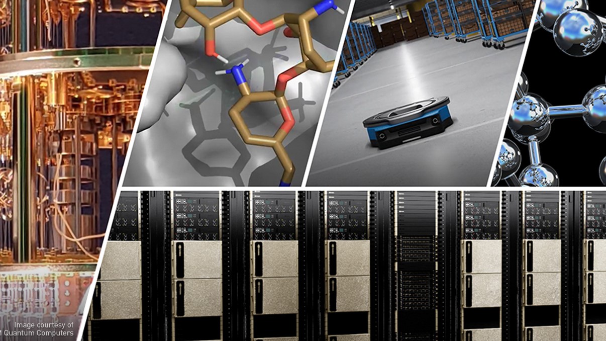
Accelerated quantum supercomputing combines the benefits of AI supercomputing with quantum processing units (QPUs) to develop solutions to some of the world’s hardest problems. Realizing such a device involves the seamless integration of one or more QPUs into a traditional CPU and GPU supercomputing architecture.
An essential component of any accelerated quantum supercomputer is a programming model to interface with it. This must be highly optimized to not only run truly hybrid quantum-classical applications but simultaneously manage control of QPU hardware. This involves orchestrating tasks such as real-time quantum error correction (QEC), making the development of performant and scalable hybrid applications extremely challenging.
The open-source NVIDIA CUDA-Q platform provides precisely such a programming model, capable of helping researchers and developers solve the challenges in implementing accelerated quantum supercomputing.
At SC24, NVIDIA announced CUDA-QX: an extension of CUDA-Q composed of optimized libraries that deliver CUDA-Q’s powerful programming model directly to the key challenges that researchers face when exploring useful quantum computing.
CUDA-QX provides optimized kernels and APIs for key quantum computing primitives (Figure 1). This lowers the threshold for researchers and developers to access CUDA-Q’s GPU acceleration, leaving you with more time to focus on novel science and application development rather than code optimization. By seamlessly integrating AI supercomputing tools into quantum research workflows, CUDA-QX catalyzes future quantum computing breakthroughs.

Figure 1. CUDA-QX architecture
This post introduces the first two CUDA-QX libraries:
- CUDA-Q QEC: Accelerates quantum error correction (QEC) research.
- CUDA-Q Solvers: A set of optimized quantum solvers for tackling domain-specific problems, such as quantum chemistry.
Examples using both are provided throughout this post, highlighting how these libraries can quickly accelerate research and application development.
CUDA-Q QEC
One of the greatest challenges standing between today’s QPUs and developing useful quantum computers is noisy qubits. Useful fault-tolerant quantum computing employs QEC to identify, track, and correct errors. This is an extremely challenging task, given the complexity of QEC codes and the stringent real-time processing requirements to decode them.
The CUDA-Q QEC library enables the seamless integration of accelerated QEC primitives into CUDA-Q workflows. You can now make use of standard QEC codes and decoders provided with CUDA-QX, or swap out your own, providing the flexibility necessary for agile research.
This also makes CUDA-Q QEC the ideal tool for experimenting with how AI algorithms can be deployed for QEC and simulating their performance at scale.
CUDA-Q QEC at work: code capacity noise models
A use case well suited to the CUDA-Q QEC library is predicting logical error rates corresponding to a QEC code and decoder pair, under code capacity assumptions.
Logical errors are catastrophic for QEC codes and result in a failure to preserve quantum data. Simulation with CUDA-Q QEC can help understand how the frequency of logical errors relates to QEC code and decoder selection under various conditions.
The first step before using CUDA-Q QEC is to install CUDA-QX and import the necessary libraries.
import numpy as np
import cudaq_qec as qec
Next, select a QEC code to study. CUDA-Q QEC has several built-in options such as the Surface and Steane codes, but you can also define your own QEC code and insert it into the same workflow.
steane = qec.get_code("steane")
The parity check matrix is defined by sets of stabilizer operators that can be measured to determine an error syndrome, from which error locations can be inferred. You can use CUDA-Q QEC to extract this parity check matrix for the Steane code.
For CSS codes like the Steane code, select the full code or just the parity check matrices that correct bit flip (X) or phase flip (Z) errors. Similarly, the mappings that determine how logical qubit states are redundantly represented within the Steane code can also be extracted.
Hz = steane.get_parity_z()
Hx = steane.get_parity_x()
H = steane.get_parity()
observable  = steane.get_observables_z()
The final step before running any analysis is to define a decoder, an algorithm that calculates a guess for error locations based on the error syndrome data obtained from parity check measurements as the code progresses.
You can construct a decoder based on your decoder selection and the parity check matrix. You can also input a custom decoder or use one of the readily available methods built into the QEC library. In this example, a lookup table (LUT) decoder is used for the Steane decoder that is predefined in CUDA-Q QEC.
decoder = qec.get_decoder("single_error_lut", Hz)
A noiseless result is the 0 bitstring, corresponding to no change in the initial logical state. To simulate the performance of this QEC coder/decoder pair, we used a simple model for introducing errors. We introduced a bit flip error to any given data qubit with probability p=0.1.
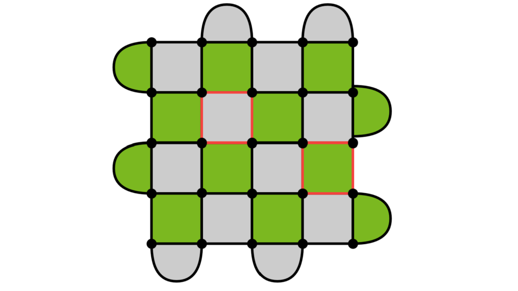
Figure 2. Schematic representation of a code capacity analysis with the Steane code
The code capacity procedure is used to assess the performance of the QEC coder/decoder pair. This is outlined in the following code example and shown in Figure 2. The procedure iterates over several shots, each corresponding to a random noisy data bitstring. The data bitstring is used to compute error syndromes, decode them, and determine if a logical state flip occurred.
In a real quantum computation, only error syndromes are accessible as any other observations of data qubits would jeopardize the encoded logical states. However, in this simulated procedure, more detailed data is available for analysis. This can be used to assess whether the decoder’s predictions of a logical state flip actually correspond to real logical flips.
If the decoder makes an incorrect prediction, then a logical error occurs, which can be recorded. The percent of shots where the decoder fails to match the actual data is the logical error rate.
# Probability of a data qubit bit flip error
p = 0.1


nShots = 10
nLogicalErrors = 0

for i in range(nShots):

    # Generate noisy data
    data = qec.generate_random_bit_flips(Hz.shape[1], p)

    # Calculate which syndromes are flagged
    syndrome = Hz@data % 2

    # Decode syndromes to determine predicted observables
    result = decoder.decode(syndrome)
    data_prediction = np.array(result.result, dtype=np.uint8)
    predicted_observable = observable@data_prediction % 2

    # Determine actual observables directly from the data
    actual_observable = observable@data % 2

    # Add to counter if logical error occurred
    if (predicted_observable != actual_observable):
        nLogicalErrors += 1

# Print the logical error rate
print(nLogicalErrors/nShots)
For convenience, you can also generate the code capacity procedure performed explicitly in this code example using a single function call.
syndromes, data = qec.sample_code_capacity(Hz, nShots, p).
The results from a code capacity exercise can be extremely useful and elucidate how physical error rates impact logical error rates.
Figure 3 shows code capacity results with the physical error rate varied. Such an analysis can be extended to circuit-level noise models to study sub-threshold scaling and identify detailed requirements on physical error rates to provide logical error rates suitable for given applications.

Figure 3. Code capacity results for the Steane code
The most convenient way to perform a circuit-level noise analysis of a QEC code is to call the sample_memory_circuit function, providing the QEC code and a noise model. The analysis also changes slightly and the number of QEC rounds must be specified along with the number of shots, or syndromes, generated with each round.
syndromes, data = qec.sample_memory_circuit(steane, numShots, numRounds, noise=noise)
The sample_memory_circuit function is compatible with custom QEC codes as long as you provide sufficient mappings to produce the correct stabilizer circuits, a procedure handled in the background for built-in codes like the Steane code.
For more information about CUDA-Q QEC usage, including C++ implementations, and a full circuit-level noise modeling workflow, see the CUDA-Q QEC documentation.
CUDA-Q Solvers
The CUDA-Q Solvers library consists of opaque methods to easily accelerate several standard quantum applications including the variational quantum eigensolver (VQE), ADAPT-VQE, and QAOA.
Though solvers are ubiquitous across many quantum applications, chemistry is one of the most frequently deployed and promising use cases. CUDA-Q Solvers is currently being used in collaboration with GE Vernova Advanced Research to simulate energy materials.
Given the importance of chemistry applications, the following sections walk you through a representative example demonstrating the utility of CUDA-Q Solvers for preparing an ADAPT-VQE simulation of a nitrogen molecule with an active space.
CUDA-Q Solvers at work: Preparing a molecule with an active space
Many quantum algorithms require classical preprocessing steps before execution on a QPU. This is particularly true for chemistry applications, where preliminary classical computations are generally necessary to prepare an initial state.
Large simulations must often make use of a so-called active space approximation to reduce the resources required to model a molecule’s electronic structure on a quantum computer. The following example walks you through building an active space with the CUDA-Q Solvers library before ADAPT-VQE is applied.
The first step is to install CUDA-QX and import the necessary libraries:
import cudaq, cudaq_solvers as solvers
import numpy as np
from scipy.optimize import minimize
Next, prepare a molecule using create_molecule. This accepts standard inputs that may be familiar from most quantum chemistry packages, such as geometry, basis set, charge, and multiplicity.
geometry=[('N', (0.0, 0.0, 0.5600)), ('N', (0.0,0.0, -0.5600))]
molecule = solvers.create_molecule(geometry,
                                            'sto-3g',    #basis set
                                            0,           #charge
                                            0,           #multiplicity
                                            nele_cas=2,
                                            norb_cas=3,
                                            ccsd=True,
                                            casci=True,
                                            verbose=True)
To specify an active space, set the number of electrons and orbitals with nele_cas and norb_cas, respectively. Setting ccsd or casci to True also computes these energies classically with the active space when the molecule is initialized. Print each computed energy with print(molecule.energies).
CUDA-Q Solvers provide additional flexibility for improving active space computations with different orbitals. For more information about examples using MP2 natural orbitals and CASSCF orbitals, see the CUDA-QX documentation.
CUDA-Q Solvers at work: accelerating ADAPT-VQE
Adaptive Derivative-Assembled Pseudo-Trotter VQE (ADAPT-VQE) is a solver technique that builds an ansatz iteratively from a predefined operator pool, which can more efficiently converge to predict the ground state energy (Figure 4). The CUDA-Q Solvers library makes it easy to use and accelerate ADAPT-VQE.
Figure 4. ADAPT-VQE procedure (Source: Quantifying the effect of gate errors on variational quantum eigensolvers for quantum chemistry)
After defining a molecule (see the earlier Preprocessing section), you only need a couple of steps to produce an ADAPT-VQE solution. First, extract the number of electrons and qubits from the molecule.
numQubits = molecule.n_orbitals * 2
numElectrons = molecule.n_electrons
Next, the cudaqx.solvers.get_operator_pool function extracts all the operators from a common ansatz and each is multiplied by a list of initial parameters to form the complete operator pool (op_pool_uccsd). In this case, the UCCSD ansatz is used, but CUDA-Q Solvers also supports the generalized single double ansatz (GSD).
# Extract operators
operators=solvers.get_operator_pool("uccsd",
                                            num_qubits=numQubits,
                                            num_electrons=numElectrons)

# Retrieve number of operators
count=len(operators)

# Make a list of initial parameters
init_params=[0.05]*count
print(init_params)

# Make final operator pool form operators and parameters
op_pool_uccsd=[1j*coef*op for coef,op in zip(init_params, operators)]
The last step before solving is to prepare an initial Hartree-Fock state as the following CUDA-Q kernel, where a bitflip operation is used to specify the occupied orbitals in the active space.
@cudaq.kernel
def initState(q: cudaq.qview):
    for i in range(numElectrons):
        x(q[i])
The ADAPT-VQE solver takes the initial state kernel, the Jordan-Wigner Hamiltonian built with molecule.hamiltonian, and a classical optimizer, which in this case is drawn from SciPy. By default, the procedure is simulated on a single NVIDIA GPU, but you can also switch in physical QPU backends trivially.
energy, thetas, ops = solvers.adapt_vqe(initState,
                                                molecule.hamiltonian,
                                                op_pool_uccsd,
                                                optimizer=minimize,
                                                method='L-BFGS-B',
                                                jac='3-point',
                                                tol=1e-7)
print('Adapt-VQE energy: ', energy)
print('Optimum pool operators: ', [op.to_string(False) for op in ops])
CUDA-Q Solvers makes it easy to accelerate applications like ADAPT-VQE and also enables you to emulate parallel computation across multiple QPUs. You can simulate this using GPUs.
To emulate calculations running across multiple QPUs, specify the MQPU target using cudaq.set_target(‘nvidia’, mqpu=’True’) followed immediately by cuadq.mpi.initialize. The same ADAPT-VQE code described earlier can then be called, followed by cuadq.mpi.finalize.
Using this emulated multi-QPU approach, the costly gradient computation of a 16-qubit nitrogen molecule simulation (six electrons in eight orbitals) is accelerated by 4.5x, all without the need for substantial code modifications (Figure 5).

Figure 5. ADAPT-VQE gradient computation accelerated with CUDA-Q Solvers on multiple GPUs
For more information, see the full sample code for this and other examples in the CUDA-Q Solvers documentation.
Get started with CUDA-QX libraries
CUDA-QX brings AI supercomputing simulation tools within the reach of quantum researchers through out-of-the-box and highly optimized libraries. The first of a growing collection of libraries, CUDA-Q Solvers and CUDA-Q QEC set the foundation for a robust toolbox that accelerates many aspects of hybrid quantum-classical applications.
To get started using the CUDA-QX libraries, see the installation instructions and the CUDA-Q Solvers and CUDA-Q QEC documentation.
These libraries require CUDA-Q as a prerequisite. For more information, see the Local Installation topic in the NVIDIA CUDA-Q documentation.


