
As many would probably agree, the development of a winning deep learning model is an iterative process of fine-tuning both the model architecture and hyperparameters. The tuning is often based on insights about the network behavior gained by examining various data obtained in training. One such data is the output from each layer of a deep learning model’s computation graph, also known as the layer’s feature map.
Feature maps represent the features extracted by a neural network when input data has flowed to a particular layer in the network. Feature maps are typically tensors with many channels and the same number of batch items as the network input. Understanding data from feature maps of a network model can provide a lot of information on the effectiveness or deficiencies of the model, while also giving clues about how the model architecture or training parameters can be optimized to get better quality and performance.
For example, when you are working on the 3D Pose Estimation model (an autoencoder based on regressions on 6D poses with image ROI and bounding-box coordinates as inputs) in NVIDIA Isaac SDK, you train the model entirely on simulated data from Unity3D, then evaluate the model with data collected from the real world. We are keen to understand how the network responds to different types of input data at different network layers, such as simulated compared to real-world. We hope that can help us improve the sim-to-real transfer of our models.
Without tools support, the direct study of feature maps from such a large network model is difficult. This is primarily due to the sheer amount of data from feature maps, but also because of the image-based nature of the feature maps (true CV-based network models).
The good news is that NVIDIA recently released a developer tool called Feature Map Explorer (FME) and it does exactly what you are looking for.
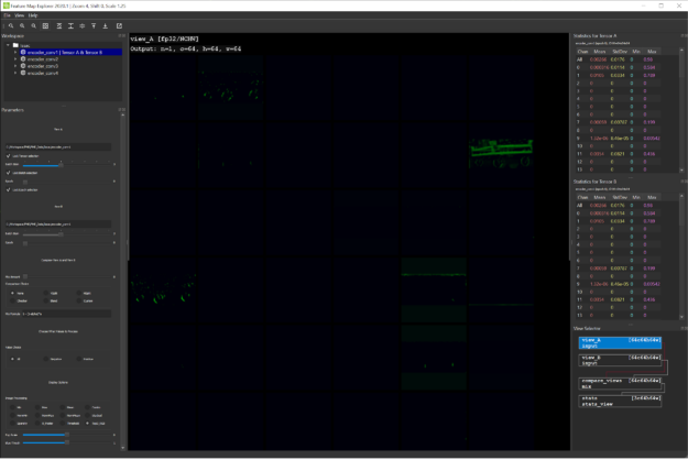
FME enables visualization of four-dimensional, image-based, feature map data in a fluid and interactive fashion, with high-level summary views and low-level channel views as well as detailed statistics information about each channel slice.
For the 3D Pose Estimation model, investigate how the convolutional layers of the encoder network (the first four layers of the network) react to different types of input before encoding it into a 128-size, latent vector space. Perform this analysis in the context of 3D pose estimation of a dolly. You first want to examine what is being learned in those layers.
Using FME to view feature maps
Using FME is straightforward. We used TensorFlow as the training framework for the 3D Pose Estimation DNN in Isaac SDK. Create a NumPy array for each of the tensors representing feature maps from the first four layers and save the arrays into .npy files by calling np.save. FME is picky about how the files are named. For more information, see How Are Feature Maps Obtained? in the NVIDIA Feature Map Explorer v2020.2 guide.
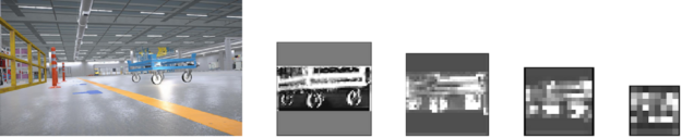
After firing up FME and pointing it to the directory containing the feature map files obtained from real-world input, you get to see a nice visualization of feature maps from each of the first four layers. Figure 2 (a) shows the full input RGB image containing the dolly whose pose must be estimated.
This input image is cropped to the dolly pixels based on the 2D bounding box and resized to a 128×128 image with black pixels as padding to retain the aspect ratio. This cropped and resized image is sent as input into the pose DNN for 3D pose estimation. Figure 2 (b), (c), (d), and (e) show the summary visualization for the feature maps of the first four encoder layers. As expected, the first couple of layers show noticeable features of the dolly. As it enters the deeper layers, the image features are encoded and non-decipherable.
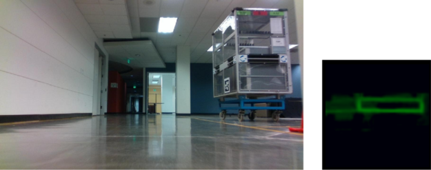
For this dolly pose estimation problem, the decoder of the network is trained to ignore the dolly wheels, as they are independent of the dolly pose. Investigating the channels of the first layer reveals channels learning only the frame of the dolly removing the wheel features as shown in Figure 3 (right). This demonstrates that the model is indeed learning to extract the dolly frame features alone. Figure 3 (left) shows the real image that is input to the pose estimation module, which is cropped and resized before sending as input into the pose network.
Comparing feature maps from different input data
FME provides two tensor views so that you can easily compare feature maps from two different sources. In this case, you are comparing feature maps from simulated input data and real-world input.
Figures 4 and 5 compare feature maps from the first convolution layer.


Figure 5 shows that features are slightly brighter and clearer for the simulated image, which is consistent with the tensor statistics shown by FME. We also observed that reflections in the simulated image result in low activations (ReLU) on the right-side vertical dolly bar.
Our key takeaway from these observations is that our network is sensitive to reflections on the dolly and could be improved by decreasing the reflectivity of the material in the training data. The comparison of the feature map activations for real data and the brightness of these activations is an indicator of the network’s confidence on sim-to-real transfer or general train-to-test data transfer. This helps track the improvements of the models during training.
Gaining insights for hyperparameter tuning
We further explored the statistics of the individual channels of the encoder convolutional layers and their visualization in FME to gain insights on the activation from different filters on inputs. In this process, we noticed that around half or more of the channels are empty from the first convolutional layer. This means that the network might have more filters than needed and so we re-trained the pose estimation model with only half the number of filters for the encoder and decoder convolutional layers. This process was captured in the following video.
We then evaluated the newly trained model on an evaluation dataset of around 1,500 images from simulation and observed an overall improvement of performance of up to 100%. We noticed significant improvements on the overall median translation and rotation errors as well.
The poorer performance of the first, larger network might be possibly due to over-fitting. Reducing the model size helped in better generalization on the test data. Evaluation metrics are run over simulated data, so the same improvement might not translate to real data. However, this exercise demonstrates that the FME tool can be helpful in hyperparameter tuning for improving neural network performance. The diagrams and tables later in this post show that the new model achieves a ~2.5x speedup while the precision improves almost 100%. These are our initial observations on sim data evaluation.
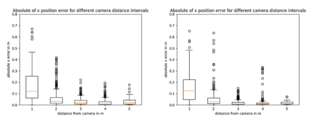
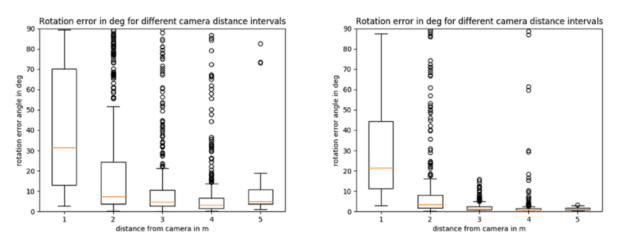
Evaluation comparisons for the dolly object
Figures 6, 7, and Table 1 show the comparisons of the box plots of absolute value of the translation and rotation errors over around 1,500 samples between the default model to the left of the images and the newly trained model with half the filters in the right of the images.
The X axis in all plots shows the different intervals for the distance of the dolly object from the camera in meters. The dolly object is fully visible above around 1.6m from the camera and the errors are larger in the first interval where camera distance is between 0 and 1m. Then, the errors reduce. Table 1 shows the overall metrics, namely the median of the absolute translation and rotation errors, and average precision comparisons for the two models. Overall, the newly trained model shows improved accuracy across both translation and rotation of the 3D pose.
| Evaluation metric | Old model | New model |
| Median x error (in m) | 0.025 m | 0.015 m |
| Median y error (in m) | 0.012 m | 0.008 m |
| Median z error (in m) | 0.05 m | 0.03 m |
| Median rotation error (in deg) | 5.1 deg | 1.6 deg |
| Average Precision(AP) * | 0.44 | 0.88 |
| Median Inference run time (on NVIDIA Jetson Xavier) | ~28 ms | ~11 ms |
*Average Precision: pose label is treated as positive if translation error is < 5cm and rotation error is < 5deg.
Conclusion
We have only used FME for a short time, but we are already seeing how easily it can help us gain valuable insights about the 3D Pose Estimation model and its ability to transfer to real data while being trained completely in simulation. This in turn has led to substantial improvements to the model. We hope that our experience with FME can also help you to improve your development experience of deep neural networks.
