
Data scientists often use the finance world as a playground for testing new techniques. Financial data has been recorded for decades, and it all takes on a numerical form, making it easy to process. Plus, there is always the chance that you create a model that makes money!
Within finance, the general goal of an investment is to maximize return (money made or lost on investment) while minimizing risk (the chance that the actual outcome differs from the predicted outcome). In short, investing money is all about the math.
This post introduces a portfolio optimization strategy that can help minimize exposure to risk. With access to a GPU, the algorithm can be sped-up by a factor up to 66x.
For retail investors, this speedup can be especially useful for frequent rebalances. Meanwhile, institutional investors can use this algorithm to manage money through a robo-advisor. Recalculating the algorithm for each unique customer’s portfolio can be computationally expensive, which can be greatly reduced by introducing a GPU.
In this post, I walk through a step-by-step guide introducing ML techniques for efficient portfolio allocation using hierarchical risk parity (HRP). This example uses Python with RAPIDS.
Choosing an algorithm for efficient financial predictions
In 1952, Harry Markowitz introduced a portfolio-optimization model known as the Modern Portfolio Theory. This model can generate a portfolio of investments that maximizes return for some given amount of risk.
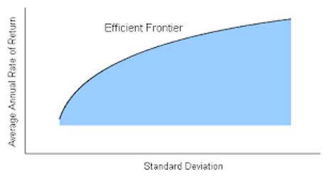
Unfortunately, the story does not end here. Markowitz’s Modern Portfolio Theory can only produce the most efficient portfolio if you know the risk and return of every equity to pick from. However, this does not always happen, because past performance is not indicative of future results.
What is hierarchical risk parity?
In 2016, Marcos López de Prado introduced HRP in his paper, Building Diversified Portfolios that Perform Well Out-Of-Sample. The idea behind this algorithm is to use machine learning techniques so that equities only have to compete with similar equities for spots in the portfolio.
For example, Verizon stock is highly correlated with AT&T. Therefore, Verizon competes for representation only against stocks like AT&T instead of against all equities in every sector.
Step-by-step guide to portfolio allocation with HRP
For the rest of this post, I focused on implementing HRP on RAPIDS and then comparing its performance to other common techniques.
Acquire data
In this post, I used daily adjusted close data from every security in the NASDAQ and NYSE over the period November 2018 to November 2021. This dataset was obtained through scripts from the NVIDIA/fsi-samples GitHub repo
For hardware, I used an i7 CPU with an NVIDIA Quadro 8000 GPU. For software, I used Python 3.9 with RAPIDS 22.02.
Wrangle data
Begin by reading in the datasets and aggregating them into a dataframe called m. Drop any equities with null values.
import cudf
m1 = cudf.read_csv("MVO3.2021.11/NASDAQ/prices.csv")
m2 = cudf.read_csv("MVO3.2021.11/NYSE/prices.csv")
m = cudf.concat([m1, m2], axis = 1)
m = m.dropna(axis = 1)
Some of the securities behave poorly: some stay flat for years, others contain non-positive values. Remove these bad securities.
data = m.values  # data.shape = (days, nAssets)
days = data.shape[0]
logRetAll = cp.log(data[1:, :]/data[:-1, :])
moveMask = cp.count_nonzero(logRetAll, axis = 0) > (days * 0.9)  # Require that each security moves day to day at least 90% of the time
positiveMask = data.min(axis = 0) > 0  # Require that all the data is positive
mask = moveMask & positiveMask
data = data[:, mask]
logRetAll = logRetAll[:, mask]
Next, split m into two parts: a training and testing period. The training period is from November 2018 to November 2020, while the testing occurs from November 2020 to November 2021.
split = int(days*2/3)
train = data[:split, :]
test = data[split:, :]
As a result, you obtain the correlation and covariance matrices using built-in cuDF methods after creating a log returns matrix for the training data, as opposed to time series data.
# Obtain training cov/corr
logRetTrain = logRetAll[:split - 1, :]
corrTrain = cp.corrcoef(logRetTrain, rowvar = False)
covTrain = cp.cov(logRetTrain, rowvar = False) * 252  # Annualized covariance
Perform clustering
To cluster equities together, define a metric that gives the distance between two equities:
\(D = \sqrt{\frac{1}{2}(1-corr)}\)
As correlation has a range of [-1, 1], you see that \(D\) has the range [0, 1] where \(D(x,y) = 0\) implies that \(x\) and \(y\) are perfectly correlated, and if \(D(x,y)=1\), then \(x\) and \(y\) are perfectly uncorrelated.
For the full proof that \(D\) is a distance metric, see the López de Prado paper.
D = cp.sqrt(0.5 * (1 - corr))
Now that you can calculate the distance between two equities, cluster them so that like equities are clustered together.
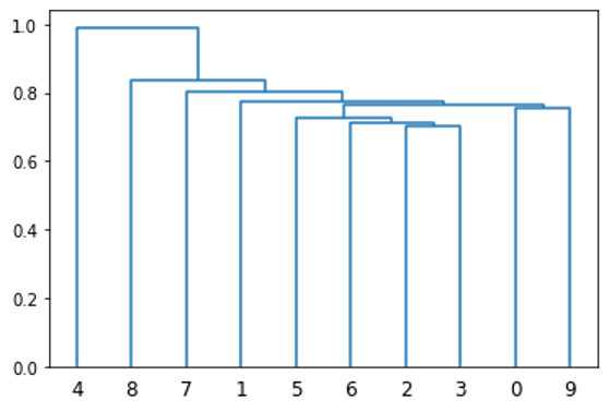
Each item is placed in its own cluster, and the two closest clusters are joined together. Then, recalculate the distance between this new cluster and all other clusters. Again, you combine the two closest clusters together. This process is repeated until there is only one cluster. One way to visualize this clustering is with a dendrogram.
from scipy.cluster.hierarchy import linkage, dendrogram
dendrogram(linkage(D[:10, :10].get()));
cuML has a built-in method to perform this function, which is used in the following code example. This is much faster than the linkage function from scipy, which performs similar functionality.
from cuml import AgglomerativeClustering as AC
# Create single linkage cluster using the Euclidean metric
def cluster(D):
    model=AC(affinity='l2', connectivity='pairwise', linkage='single')
    model.fit(D);
    return model.children_
cluster() outputs a 2 x N matrix where N is the number of equities in \(D\). The indices [0, i] and [1, i] represent the indices of the clusters joined for the i-th iteration.
Use matrix seriation
Next, produce an ordering from this clustering, which places like securities near each other. For example, the x-axis of Figure 2 provides an ordering of the first 10 stocks based on their clustering. This is done using an iterative implementation of matrix seriation, which is a common technique frequently used in archaeology.
def seriation(Z):
    N = Z.shape[1]
    stack = [2*N-2]
    res_order = []
    while(len(stack) != 0):
        cur_idx = stack.pop()
        if cur_idx < N:
            res_order.append(cur_idx)
        else:
            stack.append(int(Z[1, cur_idx-N]))
            stack.append(int(Z[0, cur_idx-N]))
    return res_order
Figure 3 shows the resulting correlation matrices.
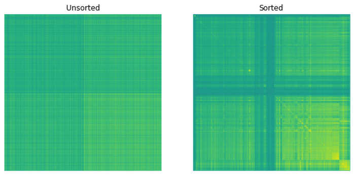
In Figure 3, you can observe patterns that emerge within the matrix when you apply your ordering to the correlation matrix. This indicates that similar equities are close to each other.
Assign weights
Finally, assign weights to the stocks. This is done through a recursive algorithm.
Split the sorted covariance matrix in half, calculating an adjusted amount of risk for each half, and then assigning weights to each half based on inverse variance portfolio (IVP) methodology. These steps are then repeated for each half.
IVP results in weights that are inversely proportional to the amount of risk, or variance, of the stock. That is, a high risk stock has low representation while a low risk stock has high representation.
Both HRP and IVP are risk-parity algorithms: they only take risk into account based on past performance.
def recursiveBisection(V, l, r, W):
    #Performs recursive bisection weighting for a new portfolio

    #V is the sorted correlation matrix
    #l is the left index of the recursion
    #r is the right index of the recursion
    #W is the list of weights

    if r-l == 1: #One item
        return W
    else:
        #Split up V matrix
        mid = l+(r-l)//2
        V1 = V[l:mid, l:mid]
        V2 = V[mid:r, mid:r]

        #Find new adjusted V
        V1_diag_inv = 1/cp.diag(V1)
        V2_diag_inv = 1/cp.diag(V2)
        w1 = V1_diag_inv/V1_diag_inv.sum()
        w2 = V2_diag_inv/V2_diag_inv.sum()
        V1_adj = w1.T@V1@w1
        V2_adj = w2.T@V2@w2

        #Adjust weights
        a2 = V1_adj/(V1_adj+V2_adj)
        a1 = 1-a2
        W[l:mid] = W[l:mid]*a1
        W[mid:r] = W[mid:r]*a2
        W = recursiveBisection(V, l, mid, W)
        W = recursiveBisection(V, mid, r, W)
        return W
Analyze weights
You now have all of the tools necessary to perform HRP. See how it performs!
#Obtain the final weights and plot them
N = len(res_order)
V = covTrain[res_order, :][:, res_order]
W_tmp = recursiveBisection(V, 0, N, cp.ones(N))
W = cp.empty(len(W_tmp))
W[res_order] = W_tmp
plt.plot(W.get())
plt.xlabel("Security Index")
plt.ylabel("% allocation")
plt.title("HRP Allocation")
plt.plot();
After applying the listed methods, you end up with a variable W that represents the weighting of each security.
Figure 4 displays the results.
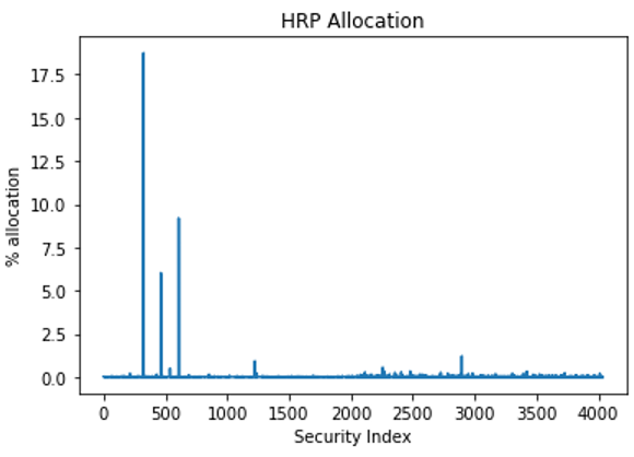
This graph is difficult to read. You can truncate it so that only securities with a weight greater than 1% are shown (Figure 5).
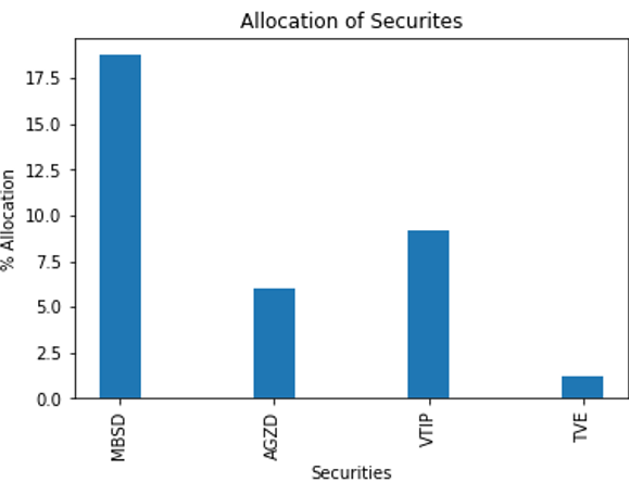
As a sanity check, Figure 6 shows how the top picks performed over the training period. You are looking to make sure that the securities have a relatively low volatility.
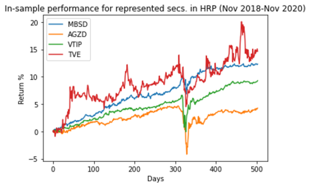
Figure 7 displays the performance of the entire portfolio over the testing period.

Compare against other portfolios
You can compare this performance to that of Modern Portfolio Theory. For this iteration, I chose to maximize the Sharpe ratio: a metric to track the performance of a portfolio.
\(\frac{return-r_f}{risk}\)
In this formula, \(r_f\) is the risk-free rate of return. In the finance world, risk is defined as \(\sqrt{w \Sigma w}\) where \(\Sigma\) is the covariance matrix. This way, both the risk and return of a portfolio are folded into the metric.
Use scipy to perform numerical optimization.
from scipy.optimize import *
from scipy.optimize import *
def MPT(cov, R):
        cons = [{'type': 'eq', 'fun': lambda x: sum(x) - 1}, #sum(w)==1",
                {'type': 'ineq', 'fun': lambda x: x}] #each weight >=0 (no short selling)"
        res = minimize(lambda x: -(x@R-1.025)/sqrt(x.T@cov@x), x0=np.ones(len(R))/len(R), constraints=cons) #Minimize risk"
        return res.x
This is a complex numerical optimization problem, especially considering that you have over 4,000 assets. Shrink this to 278 securities by requiring that each must have a Sharpe ratio greater than 1. This cutoff is arbitrary, but masking is recommended to reduce runtime.
W_MPT = cp.zeros(nAssets)
sharpeTrain = (trainRetAll - 1.025) / (cp.std(logRetTrain, axis = 0) * math.sqrt(252))  # Annualized sharpe
covnp = covTrain[sharpeTrain > 1, :][:, sharpeTrain > 1].get()  # Numpy version of covariance matrix over training period, masked
Rnp = trainRetAll[sharpeTrain > 1].get()  # Return of all stocks over the training period, masked, in numpy
W_MPT[sharpeTrain > 1] = MPT(covnp, Rnp, 1+i/100)
You can also generate weights for the inverse variance portfolio.
invVarTrain = 1 / cp.var(logRetTrain, axis = 0)
W_IVP = invVarTrain / invVarTrain.sum()
Lastly, generate some random portfolios, which choose 15 different securities, and allocate a random amount to each one. This simulates a portfolio that an uninformed retail investor might choose.
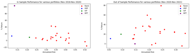
Figure 8 shows the outcomes of all portfolios.
For the preceding portfolios, you generate the Sharpe ratios in the following table.
| Train (Nov 2018 – Nov 2020) | Test (Nov 2020 – Nov 2021) | |
| Median of Random Portfolios | 0.01 | 0.97 |
| HRP | 0.91 | 1.51 |
| IVP | 0.35 | 1.83 |
| MPT | 7.51 | -0.18 |
While MPT has a high Sharpe ratio during the training sample, it turns negative during the training period, implying that the portfolio underperforms the risk-free rate of 2.5%. This demonstrates what is known as Markowitz’s curse: While it performs optimally in-sample, it oftentimes falls flat out-of-sample.
Further, while IVP has a higher Sharpe ratio than MPT over the testing period, remember that both of these methodologies are risk-parity portfolios. They aim to minimize risk and do not take return into account. It may be more pertinent to notice that over the testing period HRP has a 5.5% risk, while IVP has a 9.4% risk.
Analyze speed
One other thing to analyze is the runtime compared to a CPU. You can re-create the algorithm by using libraries such as SciPy, pandas, or NumPy instead of RAPIDS.
As the number of securities that you analyze increases, the amount of computing power required increases. This also increases the capability for parallelization, which can be captured by a GPU.
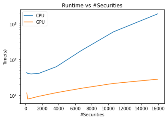
For the maximum number of securities, you achieve a speedup of 66x by running on a GPU over a CPU! Even in the worst case, you still obtain a 4x speedup.
Key learnings on HRP
Even though HRP was initially created to demonstrate how machine learning can be used in portfolio optimization, it has been shown to result possibly in less risk when compared to inverse variance and a higher Sharpe ratio than modern portfolio theory. López de Prado further backs this up in his Building Diversified Portfolios that Outperform Out of Sample paper, demonstrating lower drawdowns and variance for synthetic data.
Investors may turn to HRP when looking for ways to manage risk or to combine with other financial techniques to reduce risk for some requested rate of return.
With help from the GPU speedup that RAPIDS provides, HRP can be a viable portfolio optimization tool for a comparatively low computation cost.
