
Machine learning (ML) is increasingly used across industries. Fraud detection, demand sensing, and credit underwriting are a few examples of specific use cases.
These machine learning models make decisions that affect everyday lives. Therefore, it’s imperative that model predictions are fair, unbiased, and nondiscriminatory. Accurate predictions become vital in high-risk applications where transparency and trust are crucial.
One way to ensure fairness in AI is to analyze the predictions obtained from a machine learning model. This exposes disparities and provides the opportunity to take corrective actions to diagnose and rectify the underlying cause.
Explainable AI (XAI) is a field of Responsible AI dedicated to studying techniques that explain how a machine learning model makes predictions. These explanations are human-understandable, enabling all stakeholders to make sense of the model’s output and make the necessary decisions. SHAP is one such technique used widely in industry to evaluate and explain a model’s prediction.
This post explains how you can train an XGBoost model, implement the SHAP technique in Python using a CPU and GPU, and finally compare results between the two. By the end of the post, you should be able to answer the following questions:
- Why is it crucial to explain machine learning models, especially in high-stakes decisions?
- How do we differentiate between Interpretable and Explainable techniques?
- What is the SHAP technique, and how is it used to explain a model’s predictions?
- What is the advantage of GPU-accelerated SHAP?
Explainability versus interpretability
In the context of artificial intelligence and machine learning, it is helpful to distinguish explainability from interpretability. The terms have distinct meanings but are often used interchangeably.
In the seminal paper, Psychological Foundations of Explainability and Interpretability in Artificial Intelligence, the researchers at the US National Institute of Standards and Technology (NIST) have proposed the following definitions of explainability and interpretability:
Explanability
Explainability is a low-level, detailed mental representation that seeks to describe some complex processes. An explanation describes how some model mechanism or output came to be.
Interpretability
Interpretability is a high-level, meaningful mental representation that contextualizes a stimulus and leverages human background knowledge. An interpretable model should provide users with a description of what a data point or model output means in context.
In addition, according to Explanation in Artificial Intelligence: Insights from the Social Sciences, interpretability refers to the degree to which humans can understand and trust an ML model’s predictions.
Overview of explanation methods
The approaches to explaining model predictions can be broadly divided into model-specific and post-hoc techniques.
Model-specific
Algorithms like generalized linear models, decision trees, and generalized additive models are designed to be interpretable. These are called glassbox models because it is possible to trace and reason how a prediction was made. The techniques used to explain such models are model-specific because each method is based on some specific model’s internals. For instance, the interpretation of weights in linear models counts toward model-specific explanations.
Post-hoc
Post-hoc explainability techniques, as the name suggests, are applied after a model has been trained. Some well-known post-hoc techniques include SHAP, LIME, and Partial Dependence Plots. These are model agnostic. They work by treating the model as a BlackBox and assume they only have access to the model’s inputs and outputs. This makes them beneficial for complex algorithms, like boosted trees and deep neural nets, which are not explainable through model-specific techniques.
This post focuses on SHAP, a post-hoc technique for explaining model predictions.
Using the SHAP technique to explain models
SHAP is an acronym for SHapley Additive Explanations. It is one of the most commonly used post-hoc explainability techniques. SHAP leverages the concept of cooperative game theory to break down a prediction to measure the impact of each feature on the prediction.
Shapley values are defined as the average marginal contribution of a feature value across all possible feature coalitions. A technique with origins in economics and game theory, Shapley values assign fair payouts to players in a coalition depending upon their contribution to the total gain. Translating this into a machine learning scenario means assigning importance to features in a model depending on their contribution to the model’s prediction.
SHAP unifies several approaches to generate accurate local feature importance values using Shapley values which can then be aggregated to obtain global explanations. SHAP values interpret the impact on the model’s prediction of a given feature having a specific value, compared to the prediction we’d make if that feature took some baseline value. A baseline value is a value that the model would predict if it had no information about any feature values.
SHAP is one of the most widely used post-hoc explainability technique for calculating feature attributions. It is model agnostic, can be used both as a local and global feature attribution technique and has credible theoretical support from economics. Additionally, a variant of SHAP for tree based models reduces the computation time considerably, thereby helping users to gain insights from models quickly.
The following section provides an example of how to use the SHAP technique.
Step 1: Training an XGBoost model and calculating SHAP values
Use the well-known Adult Income Dataset to perform the following :
- Train an XGBoost model on the given dataset to predict whether a person earns more than $50K a year. Such data could be helpful in various use cases like target marketing.
- Compute the SHAP values to explain the individual feature contributions.
- Visualize and interpret the SHAP values.
Installation
SHAP can be installed using its stand-alone Python package called shap available on GitHub:
pip install shap

or
conda install -c conda-forge shap
SHAP is also inherently supported by popular algorithms like LightGBM, and XGBoost, and several R packages.
Setting up the environment
Start by setting up the environment and importing the necessary libraries:
import numpy as np
import pandas as pd

# Visualization Libraries
import matplotlib.pyplot as plt
%matplotlib inline

## Machine learning packages
from sklearn.model_selection import train_test_split
import xgboost as xgb

## Model Interpretation package
import shap
shap.initjs()

# Ensuring Reproducibility
SEED = 12345

# Ignoring the warnings
import warnings
warnings.filterwarnings(action = "ignore")
Dataset
This dataset comes from the UCI Machine Learning Repository Irvine and is available on Kaggle. It contains information about the demographic information of people based on census data. The dataset has attributes such as education, and hours of work per week, age, and so on.
The shap library ships with some commonly used datasets, including the preprocessed version of the Adult Income Dataset used below.
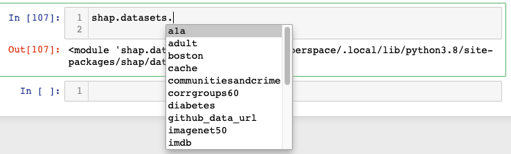
X,y = shap.datasets.adult()
X_view,y_view = shap.datasets.adult(display=True)
X_view.head()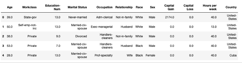
As shown above, the dataset consists of various predictor variables like Age, Work class, and Education, plus one target variable. The target variable is True if a person earns >$50K annually and False if the earned income is ≤$50K. After ensuring the dataset is preprocessed and clean, proceed with the model training.
Training an XGBoost model
XGBoost performs exceptionally well for tabular datasets and is very popular in the machine learning community. To begin, split the dataset into train and validation sets.
# create a train/test split
X_train, X_valid, y_train, y_valid = train_test_split(X, y, test_size=0.2, random_state=7)
Next, train an XGBoost model on the training data for 5K boosting rounds.
# read in the split dataset into an optimized data structure called Dmatrix required by XGBoost
dtrain = xgb.DMatrix(X_train, label=y_train)
dvalid = xgb.DMatrix(X_valid, label=y_valid)

%%time
# Feed the model the global bias
base_score = np.mean(y_train)
#Set hyperparameters for model training
params = {
   'objective': 'binary:logistic',
   'eval_metric': 'logloss',
   'eta': 0.01,
   'subsample': 0.5,
   'colsample_bytree': 0.8,
   'max_depth': 5,
   'base_score': base_score,
   'seed': SEED
}
# Train using early stopping on the validation dataset.
watchlist = [(dtrain, 'X_train'), (dvalid, 'X_test')]
model = xgb.train(params,
                       dtrain,
                       num_boost_round=5000,
                       evals=watchlist,
                       early_stopping_rounds=20,
                       verbose_eval=100)
===============================================================
Wall time: 14.3 s
The training execution takes 14.3 seconds on an Apple M1 8 Core CPU, with early stopping enabled.
See the XGBoost Parameters for more information on the configurable parameters within the XGBoost module.
Calculating SHAP values
SHAP comes in many different flavors depending on the nature of the algorithm. The most popular seem to be KernelSHAP, DeepSHAP, and TreeSHAP. While KernelSHAP is model-agnostic, TreeSHAP is only suitable for tree-based models (including the XGBoost model we just trained). Use the TreeExplainer class from the shap library to explain the entire dataset containing over 30K samples with over a thousand trees.
%%time
explainer = shap.TreeExplainer(model=model)
shap_values = explainer.shap_values(X)
================================================================
CPU times: user 4min 12s, sys: 116 ms, total: 4min 12s
Wall time: 1min 4s
Using the same hardware outlined above, the SHAP values were calculated in 1.4 minutes. Note the timing to compare them with the values obtained in the next secNow that the SHAP values have been determined, the next step is interpretation. To understand the values, shap provides several different types of visualizations like force plots, summary plots, decision plots, and more, each highlighting a specific aspect of the model. Two plots are included below.
SHAP force plot
A force plot is used to explain a single instance in the dataset. Generate a force plot for the first row in the training set and see how the different features impact the prediction. First print the ground truth label and the model’s prediction for this data instance.
classes = {0 : 'False', 1: 'True'}

# ground truth label
y[0]
=========================
False

# Model Prediction
y_pred = [round(value) for value in model.predict(dvalid)]
classes[y_pred[0]]

==========================================================
False
The ground truth label for this person is False; that is, the person earns ≤$50K annually. The model also predicts the same. Figure 2 shows a force plot for the same person giving an insight into how the various features contributed towards the model’s prediction for this particular observation.
shap.initjs()
shap.force_plot(explainer.expected_value, shap_values[0,:],X.iloc[0,:])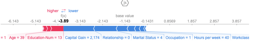
The base_value here is –1.143, while the target value for the selected sample is –3.89. All the values greater than the base value will have income ≥$50K and vice versa. For the chosen sample, the features appearing in red in Figure 2 push the prediction toward the base value while those in blue push the prediction away from the base value. It is therefore possible to infer that having a capital gain of 2,174 and relationship status of 0 negatively influences the model’s prediction for this particular person earning >$50K.
SHAP summary plot
The previous section looked at how SHAP was able to provide local explanations, or explanations specific to a single prediction. These values can be aggregated to get insights into a global view. A way to do this is by using the SHAP summary plots.
SHAP summary plots provide an overview of which features are more important for the model. This can be accomplished by plotting the SHAP values of every feature for every sample in the dataset. Figure 3 depicts a summary plot where each point in the graph corresponds to a single row in the dataset.
shap.summary_plot(shap_values_gpu, X_test)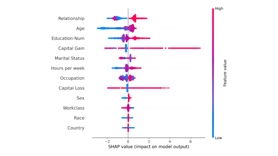
Each point in Figure 3 represents a row from the original dataset. For every point:
- The y-axis indicates the features in order of importance from top to bottom. The x-axis refers to the actual SHAP values.
- The horizontal location of a point represents the feature’s impact on the model’s prediction for that particular sample.
- The color shows whether the value of a feature is high (red) or low (blue) for any row of the dataset.
From the summary plot, it is possible to infer that ‘Relationship status’ and ‘Age’ have a higher total model impact on predicting whether a person will earn a higher income or not, as compared to other features.
Step 2: GPU-accelerated SHAP
As discussed in the previous section, TreeSHAP is a version of SHAP tailored specifically for tree ensemble models. While TreeSHAP is relatively faster, it can also face typical computation issues when the ensemble size becomes too big. In such situations, taking advantage of the GPU acceleration is advisable to speed up the process.
However, the complexity of the TreeSHAP algorithm causes difficulty when mapping to hardware accelerators. This has led to the development of GPUTreeShap, a variation of the TreeSHAP algorithm suited to work with GPUs. It is now possible to take advantage of GPU hardware while computing SHAP values, thereby speeding up the entire model explanation process.
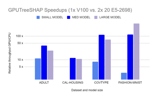
GPUTreeShap enables massively exact calculation of the shape values for tree-based algorithms. Figure 4 shows how GPUTreeSHAP provides an estimate of the gain achieved when using SHAP with GPU over CPU. According to GPUTreeShap: Massively Parallel Exact Calculation of SHAP Scores for Tree Ensembles, “With a single NVIDIA Tesla V100-32 GPU, we achieve speedups of up to 19x for SHAP values and speedups of up to 340x for SHAP interaction values over a state-of-the-art multi-core CPU implementation executed on two 20-core Xeon E5-2698 v4 2.2 GHz CPUs. We also experiment with multi-GPU computing using eight V100 GPUs, demonstrating throughput of 1.2M rows per second–equivalent CPU-based performance is estimated to require 6850 CPU cores.”
Installation
GPUTreeShap already comes integrated with the Python shap package. Another way to access GPUTreeShap is by installing the RAPIDS data science framework. This ensures access to GPUTreeShap and a host of different libraries for executing end-to-end data science pipelines entirely in the GPU.
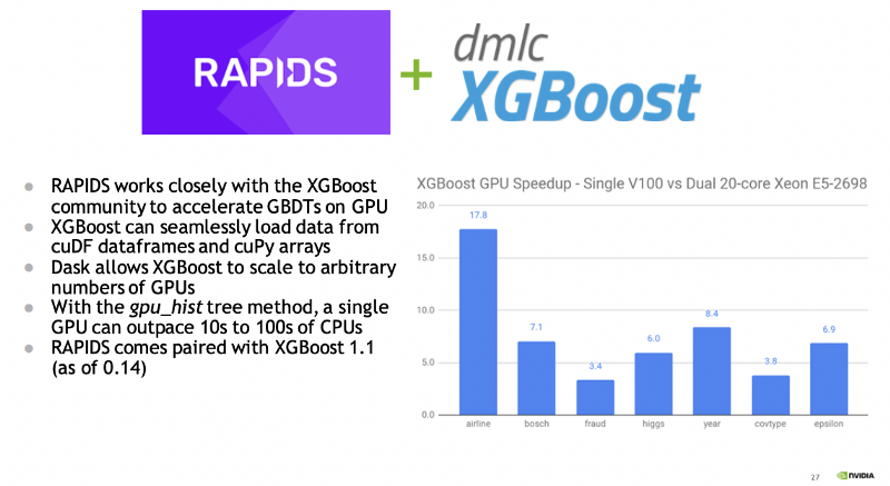
RAPIDS also comes integrated with XGBoost (as of 0.14). XGBoost was, in fact, the first popular ML Toolkit accelerated under what eventually became the RAPIDS ecosystem. Figure 5 highlights XGBoost speedup on GPU, comparing a single V100 GPU to a dual 20-core CPU.
Developers can take advantage of GPU acceleration for XGBoost and SHAP values with RAPIDS. The default open-source XGBoost packages already include GPU CUDA-capable GPUs support.
Training an XGBoost model with GPU acceleration
The previous section demonstrates who to train an XGBoost model on the Adult Income Dataset. This section repeats the same process enabled with GPU acceleration. This requires a change in the value of a single parameter called tree_method and delivers a massive decrease in the computation time.
Specify the tree_method parameter as gpu_hist, keeping all other parameters unchanged.
%%time
# Feed the model the global bias
base_score = np.mean(y_train)

#Set hyperparameters for model training
params = {
    'objective': 'binary:logistic',
    'eval_metric': 'logloss',
    'eta': 0.01,
    'subsample': 0.5,
    'colsample_bytree': 0.8,
    'max_depth': 5,
    'base_score': base_score,
    'tree_method': "gpu_hist", # GPU accelerated training
    'seed': SEED
}

# Train using early stopping on the validation dataset.
watchlist = [(dtrain, 'X_train'), (dvalid, 'X_test')]

model_gpu = xgb.train(params,
                        dtrain,
                        num_boost_round=5000,
                        evals=watchlist,
                        early_stopping_rounds=10,
                        verbose_eval=100)

=============================================================
CPU times: user 2.43 s, sys: 484 ms, total: 2.91 s
Wall time: 3.27 s
Training an XGBoost model with a single Tesla T4 GPU (available through Google Colab) helped in decreasing the training time from 14.3 seconds to just 3.27 seconds. A decrease in the compute time is beneficial since training machine learning models, especially on large datasets, can be both challenging and expensive.
Calculating SHAP values using GPU
When the GPU predictor is selected, XGBoost uses GPUTreeShap as a backend for computing shap values.
%%time
model_gpu.set_param({"predictor": "gpu_predictor"})
explainer_gpu = shap.TreeExplainer(model=model_gpu)
shap_values_gpu = explainer_gpu.shap_values(X)
==========================================================
CPU times: user 1.34 s, sys: 252 ms, total: 1.59 s
Wall time: 1.56 s
Using GPU, the computation time for calculating Shapley values decreases to 1.56 seconds, from 1.4 minutes, gaining a massive reduction in computation time. The gain would be even more prominent when the dataset involves millions of data points, which is typical in many industries.
Summary
Techniques like SHAP can make machine learning systems more trustworthy. If a model can be faithfully explained, it can be analyzed to determine whether it is fit to be deployed. This is an essential step toward inculcating trust in any technology. With GPU acceleration, it is possible to compute SHAP values faster, allowing you to gain insights into predictive models more quickly.
However, SHAP is not a silver bullet and has its own set of limitations.The main criticism of SHAP is that it can be misinterpreted. SHAP essentially helps in answering the question of why a particular observation received a prediction rather than a baseline value. This baseline value is dictated by the choice of a background dataset and can offer contrasting results if the reference dataset changes.
Consequently, the same observation can result in different SHAP values, depending on the choice of the background dataset. It is therefore important to carefully and appropriately choose background datasets keeping in mind the context of their use. It is important to understand the assumptions and trade-offs associated with explainability techniques in machine learning.
To see the code used in this post, visit parulnith/Data-Science-Articles on GitHub.
