In a new automotive application, we have used convolutional neural networks (CNNs) to map the raw pixels from a front-facing camera to the steering commands for a self-driving car. This powerful end-to-end approach means that with minimum training data from humans, the system learns to steer, with or without lane markings, on both local roads and highways. The system can also operate in areas with unclear visual guidance such as parking lots or unpaved roads. [Editor’s Note: be sure to check out the new post “Explaining How End-to-End Deep Learning Steers a Self-Driving Car“].
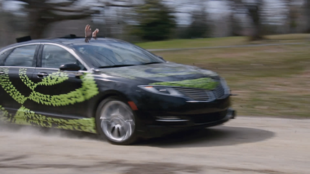
We designed the end-to-end learning system using an NVIDIA DevBox running Torch 7 for training. An NVIDIA DRIVETM PX self-driving car computer, also with Torch 7, was used to determine where to drive—while operating at 30 frames per second (FPS). The system is trained to automatically learn the internal representations of necessary processing steps, such as detecting useful road features, with only the human steering angle as the training signal. We never explicitly trained it to detect, for example, the outline of roads. In contrast to methods using explicit decomposition of the problem, such as lane marking detection, path planning, and control, our end-to-end system optimizes all processing steps simultaneously.
We believe that end-to-end learning leads to better performance and smaller systems. Better performance results because the internal components self-optimize to maximize overall system performance, instead of optimizing human-selected intermediate criteria, e. g., lane detection. Such criteria understandably are selected for ease of human interpretation which doesn’t automatically guarantee maximum system performance. Smaller networks are possible because the system learns to solve the problem with the minimal number of processing steps.
This blog post is based on the NVIDIA paper End to End Learning for Self-Driving Cars. Please see the original paper for full details.
Convolutional Neural Networks to Process Visual Data
CNNs[1] have revolutionized the computational pattern recognition process[2]. Prior to the widespread adoption of CNNs, most pattern recognition tasks were performed using an initial stage of hand-crafted feature extraction followed by a classifier. The important breakthrough of CNNs is that features are now learned automatically from training examples. The CNN approach is especially powerful when applied to image recognition tasks because the convolution operation captures the 2D nature of images. By using the convolution kernels to scan an entire image, relatively few parameters need to be learned compared to the total number of operations.
While CNNs with learned features have been used commercially for over twenty years [3],their adoption has exploded in recent years because of two important developments. First, large, labeled data sets such as the ImageNet Large Scale Visual Recognition Challenge (ILSVRC)[4] are now widely available for training and validation. Second, CNN learning algorithms are now implemented on massively parallel graphics processing units (GPUs), tremendously accelerating learning and inference ability.
The CNNs that we describe here go beyond basic pattern recognition. We developed a system that learns the entire processing pipeline needed to steer an automobile. The groundwork for this project was actually done over 10 years ago in a Defense Advanced Research Projects Agency (DARPA) seedling project known as DARPA Autonomous Vehicle (DAVE)[5], in which a sub-scale radio control (RC) car drove through a junk-filled alley way. DAVE was trained on hours of human driving in similar, but not identical, environments. The training data included video from two cameras and the steering commands sent by a human operator.
In many ways, DAVE was inspired by the pioneering work of Pomerleau[6], who in 1989 built the Autonomous Land Vehicle in a Neural Network (ALVINN) system. ALVINN is a precursor to DAVE, and it provided the initial proof of concept that an end-to-end trained neural network might one day be capable of steering a car on public roads. DAVE demonstrated the potential of end-to-end learning, and indeed was used to justify starting the DARPA Learning Applied to Ground Robots (LAGR) program[7], but DAVE’s performance was not sufficiently reliable to provide a full alternative to the more modular approaches to off-road driving. (DAVE’s mean distance between crashes was about 20 meters in complex environments.)
About a year ago we started a new effort to improve on the original DAVE, and create a robust system for driving on public roads. The primary motivation for this work is to avoid the need to recognize specific human-designated features, such as lane markings, guard rails, or other cars, and to avoid having to create a collection of “if, then, else” rules, based on observation of these features. We are excited to share the preliminary results of this new effort, which is aptly named: DAVE–2.
The DAVE-2 System
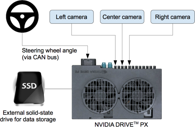
Figure 2 shows a simplified block diagram of the collection system for training data of DAVE-2. Three cameras are mounted behind the windshield of the data-acquisition car, and timestamped video from the cameras is captured simultaneously with the steering angle applied by the human driver. The steering command is obtained by tapping into the vehicle’s Controller Area Network (CAN) bus. In order to make our system independent of the car geometry, we represent the steering command as 1/r, where r is the turning radius in meters. We use 1/r instead of r to prevent a singularity when driving straight (the turning radius for driving straight is infinity). 1/r smoothly transitions through zero from left turns (negative values) to right turns (positive values).
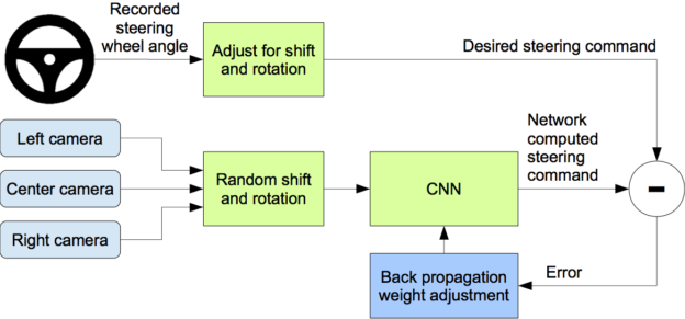
Training data contains single images sampled from the video, paired with the corresponding steering command (1/r). Training with data from only the human driver is not sufficient; the network must also learn how to recover from any mistakes, or the car will slowly drift off the road. The training data is therefore augmented with additional images that show the car in different shifts from the center of the lane and rotations from the direction of the road.
The images for two specific off-center shifts can be obtained from the left and the right cameras. Additional shifts between the cameras and all rotations are simulated through viewpoint transformation of the image from the nearest camera. Precise viewpoint transformation requires 3D scene knowledge which we don’t have, so we approximate the transformation by assuming all points below the horizon are on flat ground, and all points above the horizon are infinitely far away. This works fine for flat terrain, but for a more complete rendering it introduces distortions for objects that stick above the ground, such as cars, poles, trees, and buildings. Fortunately these distortions don’t pose a significant problem for network training. The steering label for the transformed images is quickly adjusted to one that correctly steers the vehicle back to the desired location and orientation in two seconds.
Figure 3 shows a block diagram of our training system. Images are fed into a CNN that then computes a proposed steering command. The proposed command is compared to the desired command for that image, and the weights of the CNN are adjusted to bring the CNN output closer to the desired output. The weight adjustment is accomplished using back propagation as implemented in the Torch 7 machine learning package.
Once trained, the network is able to generate steering commands from the video images of a single center camera. Figure 4 shows this configuration.

Data Collection
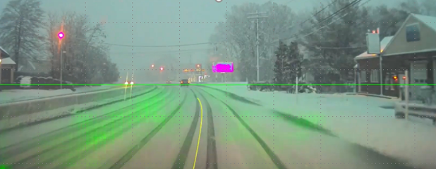
Training data was collected by driving on a wide variety of roads and in a diverse set of lighting and weather conditions. We gathered surface street data in central New Jersey and highway data from Illinois, Michigan, Pennsylvania, and New York. Other road types include two-lane roads (with and without lane markings), residential roads with parked cars, tunnels, and unpaved roads. Data was collected in clear, cloudy, foggy, snowy, and rainy weather, both day and night. In some instances, the sun was low in the sky, resulting in glare reflecting from the road surface and scattering from the windshield.
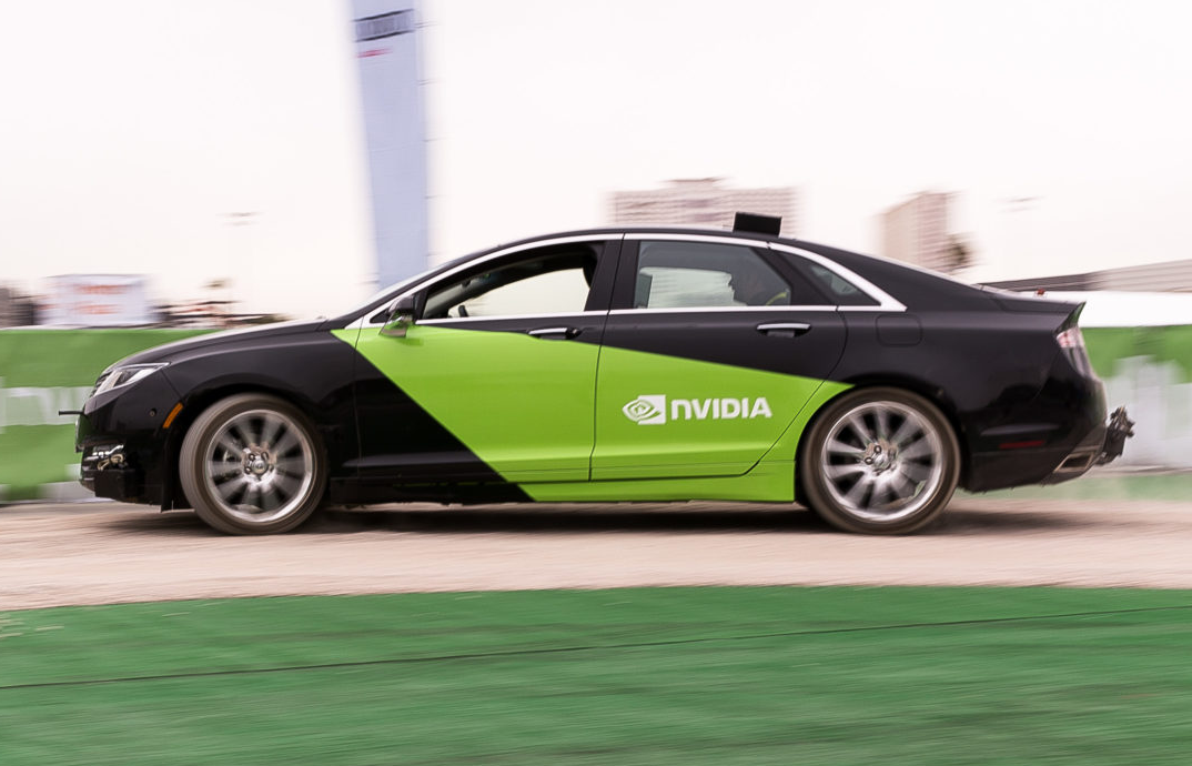
The data was acquired using either our drive-by-wire test vehicle, which is a 2016 Lincoln MKZ, or using a 2013 Ford Focus with cameras placed in similar positions to those in the Lincoln. Our system has no dependencies on any particular vehicle make or model. Drivers were encouraged to maintain full attentiveness, but otherwise drive as they usually do. As of March 28, 2016, about 72 hours of driving data was collected.
Network Architecture
We train the weights of our network to minimize the mean-squared error between the steering command output by the network, and either the command of the human driver or the adjusted steering command for off-center and rotated images (see “Augmentation”, later). Figure 5 shows the network architecture, which consists of 9 layers, including a normalization layer, 5 convolutional layers, and 3 fully connected layers. The input image is split into YUV planes and passed to the network.
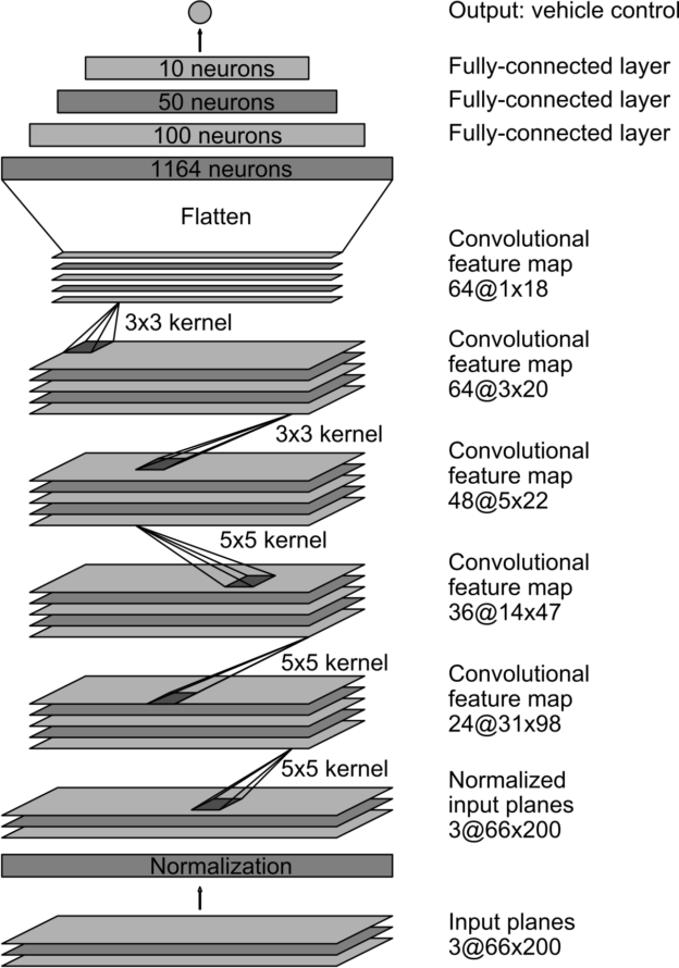
The first layer of the network performs image normalization. The normalizer is hard-coded and is not adjusted in the learning process. Performing normalization in the network allows the normalization scheme to be altered with the network architecture, and to be accelerated via GPU processing.
The convolutional layers are designed to perform feature extraction, and are chosen empirically through a series of experiments that vary layer configurations. We then use strided convolutions in the first three convolutional layers with a 2×2 stride and a 5×5 kernel, and a non-strided convolution with a 3×3 kernel size in the final two convolutional layers.
We follow the five convolutional layers with three fully connected layers, leading to a final output control value which is the inverse-turning-radius. The fully connected layers are designed to function as a controller for steering, but we noted that by training the system end-to-end, it is not possible to make a clean break between which parts of the network function primarily as feature extractor, and which serve as controller.
Training Details
Data Selection
The first step to training a neural network is selecting the frames to use. Our collected data is labeled with road type, weather condition, and the driver’s activity (staying in a lane, switching lanes, turning, and so forth). To train a CNN to do lane following, we simply select data where the driver is staying in a lane, and discard the rest. We then sample that video at 10 FPS because a higher sampling rate would include images that are highly similar, and thus not provide much additional useful information. To remove a bias towards driving straight the training data includes a higher proportion of frames that represent road curves.
Augmentation
After selecting the final set of frames, we augment the data by adding artificial shifts and rotations to teach the network how to recover from a poor position or orientation. The magnitude of these perturbations is chosen randomly from a normal distribution. The distribution has zero mean, and the standard deviation is twice the standard deviation that we measured with human drivers. Artificially augmenting the data does add undesirable artifacts as the magnitude increases (as mentioned previously).
Simulation
Before road-testing a trained CNN, we first evaluate the network’s performance in simulation. Figure 6 shows a simplified block diagram of the simulation system, and Figure 7 shows a screenshot of the simulator in interactive mode.
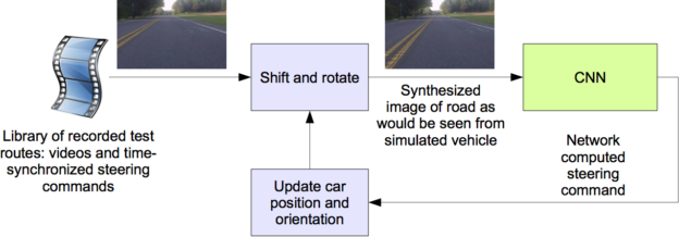
The simulator takes prerecorded videos from a forward-facing on-board camera connected to a human-driven data-collection vehicle, and generates images that approximate what would appear if the CNN were instead steering the vehicle. These test videos are time-synchronized with the recorded steering commands generated by the human driver.
Since human drivers don’t drive in the center of the lane all the time, we must manually calibrate the lane’s center as it is associated with each frame in the video used by the simulator. We call this position the “ground truth”.
The simulator transforms the original images to account for departures from the ground truth. Note that this transformation also includes any discrepancy between the human driven path and the ground truth. The transformation is accomplished by the same methods as described previously.
The simulator accesses the recorded test video along with the synchronized steering commands that occurred when the video was captured. The simulator sends the first frame of the chosen test video, adjusted for any departures from the ground truth, to the input of the trained CNN, which then returns a steering command for that frame. The CNN steering commands as well as the recorded human-driver commands are fed into the dynamic model [7] of the vehicle to update the position and orientation of the simulated vehicle.
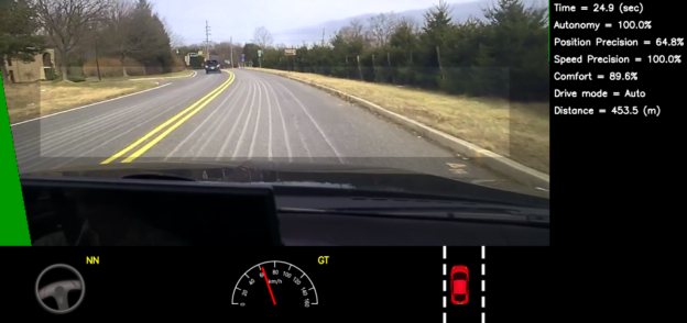
The simulator then modifies the next frame in the test video so that the image appears as if the vehicle were at the position that resulted by following steering commands from the CNN. This new image is then fed to the CNN and the process repeats.
The simulator records the off-center distance (distance from the car to the lane center), the yaw, and the distance traveled by the virtual car. When the off-center distance exceeds one meter, a virtual human intervention is triggered, and the virtual vehicle position and orientation is reset to match the ground truth of the corresponding frame of the original test video.
Evaluation
We evaluate our networks in two steps: first in simulation, and then in on-road tests.
In simulation we have the networks provide steering commands in our simulator to an ensemble of prerecorded test routes that correspond to about a total of three hours and 100 miles of driving in Monmouth County, NJ. The test data was taken in diverse lighting and weather conditions and includes highways, local roads, and residential streets.
We estimate what percentage of the time the network could drive the car (autonomy) by counting the simulated human interventions that occur when the simulated vehicle departs from the center line by more than one meter. We assume that in real life an actual intervention would require a total of six seconds: this is the time required for a human to retake control of the vehicle, re-center it, and then restart the self-steering mode. We calculate the percentage autonomy by counting the number of interventions, multiplying by 6 seconds, dividing by the elapsed time of the simulated test, and then subtracting the result from 1:
\(\text{autonomy} = (1 – \frac{\text{\# of interventions} \cdot 6 \text{[seconds]}}{\text{elapsed time[seconds]}}) \cdot 100\)
Thus, if we had 10 interventions in 600 seconds, we would have an autonomy value of
\((1 – \frac{10 \cdot 6}{600}) \cdot 100 = 90\%\)
On-road Tests
After a trained network has demonstrated good performance in the simulator, the network is loaded on the DRIVE PX in our test car and taken out for a road test. For these tests we measure performance as the fraction of time during which the car performs autonomous steering. This time excludes lane changes and turns from one road to another. For a typical drive in Monmouth County NJ from our office in Holmdel to Atlantic Highlands, we are autonomous approximately 98% of the time. We also drove 10 miles on the Garden State Parkway (a multi-lane divided highway with on and off ramps) with zero intercepts.
Here is a video of our test car driving in diverse conditions.
Visualization of Internal CNN State
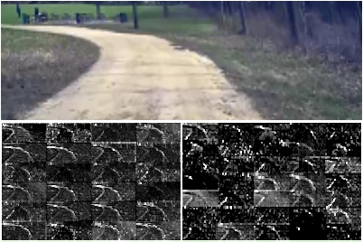
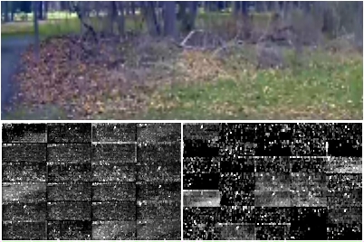
Figures 8 and 9 show the activations of the first two feature map layers for two different example inputs, an unpaved road and a forest. In case of the unpaved road, the feature map activations clearly show the outline of the road while in case of the forest the feature maps contain mostly noise, i. e., the CNN finds no useful information in this image.
This demonstrates that the CNN learned to detect useful road features on its own, i. e., with only the human steering angle as training signal. We never explicitly trained it to detect the outlines of roads, for example.
Conclusions
We have empirically demonstrated that CNNs are able to learn the entire task of lane and road following without manual decomposition into road or lane marking detection, semantic abstraction, path planning, and control. A small amount of training data from less than a hundred hours of driving was sufficient to train the car to operate in diverse conditions, on highways, local and residential roads in sunny, cloudy, and rainy conditions. The CNN is able to learn meaningful road features from a very sparse training signal (steering alone).
The system learns for example to detect the outline of a road without the need of explicit labels during training.
More work is needed to improve the robustness of the network, to find methods to verify the robust- ness, and to improve visualization of the network-internal processing steps.
For full details please see the paper that this blog post is based on, and please contact us if you would like to learn more about NVIDIA’s autonomous vehicle platform!
References
- Y. LeCun, B. Boser, J. S. Denker, D. Henderson, R. E. Howard, W. Hubbard, and L. D. Jackel. Backprop- agation applied to handwritten zip code recognition. Neural Computation, 1(4):541–551, Winter 1989. URL: http://yann.lecun.org/exdb/publis/pdf/lecun-89e.pdf.
- Alex Krizhevsky, Ilya Sutskever, and Geoffrey E. Hinton. Imagenet classification with deep convolutional neural networks. In F. Pereira, C. J. C. Burges, L. Bottou, and K. Q. Weinberger, editors, Advances in Neural Information Processing Systems 25, pages 1097–1105. Curran Associates, Inc., 2012. URL: http://papers.nips.cc/paper/ 4824-imagenet-classification-with-deep-convolutional-neural-networks. pdf.
- L. D. Jackel, D. Sharman, Stenard C. E., Strom B. I., , and D Zuckert. Optical character recognition for self-service banking. AT&T Technical Journal, 74(1):16–24, 1995.
- Large scale visual recognition challenge (ILSVRC). URL: http://www.image-net.org/ challenges/LSVRC/.
- Net-Scale Technologies, Inc. Autonomous off-road vehicle control using end-to-end learning, July 2004. Final technical report. URL: http://net-scale.com/doc/net-scale-dave-report.pdf.
- Dean A. Pomerleau. ALVINN, an autonomous land vehicle in a neural network. Technical report, Carnegie Mellon University, 1989. URL: http://repository.cmu.edu/cgi/viewcontent. cgi?article=2874&context=compsci.
- Danwei Wang and Feng Qi. Trajectory planning for a four-wheel-steering vehicle. In Proceedings of the 2001 IEEE International Conference on Robotics & Automation, May 21–26 2001. URL: http: //www.ntu.edu.sg/home/edwwang/confpapers/wdwicar01.pdf.

