To develop an accurate computer vision AI application, you need massive amounts of high-quality data. With a traditional dataset, you might spend months collecting images, getting annotations, and cleaning data. When it’s done, you could find edge cases and need more data, starting the cycle all over again.
For years, this cycle has held back AI, especially in computer vision. Lexset builds tools that enable you to generate data to solve this bottleneck. Powerful new workflows with training data can be developed and iterated as part of the AI training cycle.
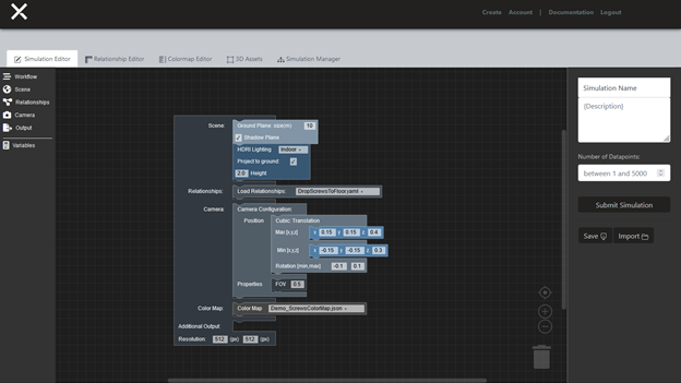
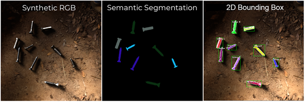
Lexset’s Seahaven platform generates fully annotated datasets, including photorealistic RGB images, semantic segmentation, and depth maps, in a matter of minutes. Iteration to improve your model’s accuracy is fast and effective. It’s not a months-long process to find data for unusual events or rare conditions anymore. Just quickly adjust your configuration and generate new data to make your model better than ever.
The synthetic data generated from Seahaven can be used to fine-tune and customize pretrained models from the NVIDIA TAO Toolkit. The TAO Toolkit, a low-code AI model development solution, abstracts the complexity of AI frameworks and enables you to create custom, production-ready models for your specific use case with transfer learning.
Reduce time and increase accuracy significantly by using both Seahaven and TAO Toolkit in creating an initial dataset. Most importantly, you can use synthetic data to quickly adapt a model to changing conditions and increased complexity.
Solution overview
For this experiment, you take a simple use case and build a computer vision model capable of finding and differentiating between a common hardware item, such as screws. You start with a simple background and introduce more complexity to show how adaptable synthetic data is to changing conditions.
We created a dataset containing images with annotations of the four screws and used the TAO Toolkit Object Detection model to get started. We used Faster R-CNN, RetinaNet, and YOLOv3.
In this post, I cover the steps required to run this sample dataset, which you can download, through Faster R-CNN. To run RetinaNet or YOLOv3, the steps are the same and are in the provided Jupyter notebook.
I also share how the Lexset synthetic data can be used in concert with model training to quickly address accuracy issues that may arise as use cases become more complex.
To make your own dataset to use with TAO Toolkit, follow the instructions at Using Seahaven and the Seahaven documentation.
To reproduce the results described, follow these main steps:
- Use a pretrained ResNet-18 model and train a ResNet-18 Faster RCNN model on Lexset’s four screws synthetic dataset.
- Use the best trained weights on the synthetic dataset and fine-tune them with 10% of the real-world four-screw dataset.
- Evaluate the best trained and fine-tuned weights on the real screws validation dataset.
- Run inference on the trained model.
Prerequisites
NVIDIA TAO Toolkit requires an NVIDIA GPU (for example, A100) and driver to use their Docker container, so you must have one to proceed.
You also need at least 16 GBs physical RAM, 50 GB of available memory, and an 8-Core. We tested on Python 3.6.9 and used Ubuntu 18.04. TAO Toolkit requires NVIDIA driver 455.xx or later.
- The tao-launcher is strictly a python3-only package, capable of running on Python 3.6.9 or 3.7 or 3.8.
- Install docker-ce by following the official Docker instructions.
- After you have installed docker-ce, follow the post-installation steps to ensure that Docker can be run without sudo.
- Install nvidia-container-toolkit.
- You must have an NGC account and an API key associated with your account. For more information about creating an NGC account and obtaining an API key, see the Installation Prerequisites section.
Download the dataset
Download the dataset from the Google Drive folder (link also provided in the notebook), which contains all the zip files for synthetic and real images of screws.
●	synthetic_dataset_without_complex_phase1.zip
●	synthetic_dataset_with_complex_phase2.zip
●	real_dataset.zip
Extract the dataset inside synthetic_dataset_without_complex_phase1.zip and real_dataset.zip into the /data directory. The dataset directory structure should look like the following:
├── real_test
├── real_train
├── synthetic_test
└── synthetic_train
TAO Toolkit supports datasets in KITTI format, and the provided dataset is already in that format. To verify it further, see KITTI file format.
Environment setup
Create a new virtual environment using virtualenvwrapper. For more information, see Virtual Environments in the Python Guide.
When you have followed the instructions to install virtualenv and virtualenvwrapper, set the Python version:
echo "export VIRTUALENVWRAPPER_PYTHON=/usr/bin/python3" >> ~/.bashrc
source ~/.bashrc
mkvirtualenv launcher -p /usr/bin/python3
Clone the repository:
git clone https://github.com/Lexset/NVIDIA-TAO-Toolkit---Synthetic-Data.git
cd tao-screws
To install the required dependencies for the environment, install the requirements.txt file:
pip3 install -r requirements.txt
Start the Jupyter notebook:
cd faster_rcnn
jupyter notebook --ip 0.0.0.0 --allow-root --port 8888
Setting up TAO Toolkit mounts
The notebook has a script to generate a ~/.tao_mounts.json file.
{
      "Mounts": [
        {
            "source": "ABSOLUTE_PATH_TO_PROJECT_NETWORK_DIRECTORY",
            "destination": "/workspace/tao-experiments"
        },
        {
         "source": "ABSOLUTE_PATH_TO_PROJECT_NETWORK_SPECS_DIRECTORY",
            "destination": "/workspace/tao-experiments/faster_rcnn/specs"
        }
    ],
     "Envs": [
         {
             "variable": "CUDA_VISIBLE_DEVICES",
             "value": "0"
         }
     ],
     "DockerOptions": {
         "shm_size": "16G",
         "ulimits": {
             "memlock": -1,
             "stack": 67108864
         },
         "user": "1001:1001"
     }
 }
The code example generates the global ~/.tao_mounts.json file at the Ubuntu home directory.
Processing the dataset into TFRecords
When the dataset is downloaded and placed in a data directory, the next step is to convert the KITTI files into the TFRecord format used by NVIDIA TAO Toolkit. Generate TFrecords for both the synthetic and real datasets. This code example from the Jupyter notebook generates TFrecords:
#KITTI trainval
!tao faster_rcnn dataset_convert --gpu_index $GPU_INDEX -d $SPECS_DIR/faster_rcnn_tfrecords_kitti_synth_train.txt \
                    -o $DATA_DOWNLOAD_DIR/tfrecords/kitti_synthetic_train/kitti_synthetic_train

!tao faster_rcnn dataset_convert --gpu_index $GPU_INDEX -d $SPECS_DIR/faster_rcnn_tfrecords_kitti_synth_test.txt \
                    -o $DATA_DOWNLOAD_DIR/tfrecords/kitti_synthetic_test/kitti_synthetic_test
The same conversion is applied on the real dataset by the next code example in the notebook.
Download the ResNet-18 convolutional backbone
On the setup of NGC CLI locally, download the convolutional backbone, ResNet-18.
!ngc registry model list nvidia/tao/pretrained_object_detection*
Run a benchmark experiment using synthetic data
The following commands start the training on synthetic data and all the logs are saved on out_resnet18_synth_amp16.log file. To see the logs, open the file or refresh the tab if the file was already opened.
!tao faster_rcnn train --gpu_index $GPU_INDEX -e $SPECS_DIR/default_spec_resnet18_synth_train.txt --use_amp > out_resnet18_synth_amp16.log
Alternatively, you can use the tail command to see the last few lines of the logs.
!tail -f ./out_resnet18_synth_amp16.log
After the training is completed on the synthetic dataset, you can evaluate the synthetically trained model on 10% synthetic validation dataset using the following commands:
!tao faster_rcnn evaluate --gpu_index $GPU_INDEX -e $SPECS_DIR/default_spec_resnet18_synth_train.txt
You see the results like the following.
mAP@0.5 = 0.9986
You also see the individual mAP scores for each class.
Fine-tuning the synthetic-trained model with real data
Now, use the best trained weights from synthetic training and perform the fine-tuning on 10% of the real-world screw dataset. The /train folder inside real_train is already at a 10% split and you can start the fine-tuning using the following commands:
!tao faster_rcnn train --gpu_index $GPU_INDEX -e $SPECS_DIR/default_spec_resnet18_real_train.txt --use_amp > out_resnet18_synth_fine_tune_10_amp16.log
Results: Improvements on 10% of the real data
Per epoch, the mAP score looks like the following data:
mAP@0.5 = 0.9408
mAP@0.5 = 0.9714
mAP@0.5 = 0.9732
mAP@0.5 = 0.9781
mAP@0.5 = 0.9745
mAP@0.5 = 0.9780
mAP@0.5 = 0.9815
mAP@0.5 = 0.9820
mAP@0.5 = 0.9803
mAP@0.5 = 0.9796
mAP@0.5 = 0.9810
mAP@0.5 = 0.9817
Fine tuning on just 10% of the real-world screw dataset improves the results quickly and the mAP score above 98%. The features learned from the synthetic dataset helped during the fine-tuning on just 10% of the real-world screw dataset.
Add a complex background in the synthetic screws validation dataset
To further validate the synthetically trained model, we added 300 more images to the complex background dataset. As the initial synthetic dataset was not taken with a complex background, the mean average precision drops significantly.
Just like the real world, as the use case becomes more complex, the accuracy suffers. When validated on images containing more complex or adversarial backgrounds, the mAP score dropped from around 98% to 83.5%.
Retrain the synthetic dataset with complex backgrounds
This is where synthetic data really shines. To mitigate the loss in mAP when validated on complex images, I generated additional images with more complex backgrounds to add to the training data. I just adjusted the backgrounds so that the new training data set was ready in a manner of seconds. After being introduced, the new dataset boosted performance by an incredible 10-12% with no additional changes.
The dataset with the complex backgrounds is inside the zip file synthetic_dataset_with_complex.zip mentioned earlier. Extract this file and replace the folders inside the /data directory with the same names to have an updated synthetic dataset with a complex background.
Average Mean Precision:
mAP= 94.97%

Increase in mAP score: 11.47%
Specifically, the accuracy of the system with complex backgrounds rose as much as 11.47%, to 94.97%, after just a few minutes of work.
Conclusion
The results showed just how effective and quick it is to iterate with synthetic data and the TAO Toolkit. Using Lexset’s Seahaven, you can generate new data in a matter of minutes and use it to resolve the accuracy issues encountered with introduced complex backgrounds.
The importance of the synthetic dataset is now clear, as the performance of the fine-tuned model on the 90% validation dataset for real-world screw data is extremely good. Use a synthetic dataset for initial feature learning when you have less actual or real-world data. Synthetic datasets can save significant time and cost while producing superior results.
I believe this is the future of computer vision development, where data production occurs in tandem with model iteration. This will give greater controls to the user and enabling you to build the best systems the world has ever seen.
Get started by downloading the Jupyter notebook and sample dataset.
To create your own data, sign up for an account with Lexset.