NVIDIA NeMo has consistently developed automatic speech recognition (ASR) models that set the benchmark in the industry, particularly those topping the Hugging Face Open ASR Leaderboard.
These NVIDIA NeMo ASR models that transcribe speech into text offer a range of architectures designed to optimize both speed and accuracy:
- CTC model (nvidia/parakeet-ctc-1.1b): This model features a FastConformer encoder and a softmax prediction head. It’s non-autoregressive, meaning future predictions do not depend on the previous ones, enabling fast and efficient inference.
- RNN-T model (nvidia/parakeet-rnnt-1.1b): This transducer model adds a prediction and joint network to the FastConformer encoder, making it autoregressive—each prediction depends on the previous prediction history. Due to this property, there is a common misconception that RNN-T models are slow for GPU inference and better suited to CPUs.
- TDT model (nvidia/parakeet-tdt-1.1b): Another transducer model, but trained with a refined transducer objective called token-and-duration transducer (TDT). While still autoregressive, it can perform multiple predictions at each step, making it faster at inference.
- TDT-CTC model (parakeet-tdt_ctc-110m): This is a hybrid variant of transducer and CTC decoders, bringing both decoders for faster convergence during training. It enables training only one model for two decoders.
- AED model (nvidia/canary-1b): Attention-encoder-decoder (AED) model, also based on the FastConformer, is autoregressive and offers the highest accuracy (lowest word error rate, or WER) at the cost of additional computation.
Previously, these models faced speed performance bottlenecks such as casting overheads, low compute intensity, and divergence performance issues.
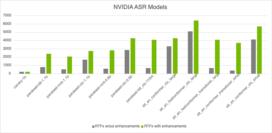
In this post, you’ll discover how NVIDIA boosted the inference speed of NeMo ASR models by up to 10x (Figure 1) through key enhancements like autocasting tensors to bfloat16, the innovative label-looping algorithm, and the introduction of CUDA Graphs available with NeMo 2.0.0.
Overcoming speed performance bottlenecks
This section dives into how NVIDIA ASR models overcame various speed performance bottlenecks, from casting overheads to batch processing optimization, low compute intensity, and divergence performance issues.
Casting overheads from automatic mixed precision
From the early days of NeMo, inference has been performed within torch.amp.autocast context manager. This automatically casts float32 weights to float16 or bfloat16 before matrix multiplications, enabling the use of half precision tensor core operations. Under the hood, automatic mixed precision (AMP) maintains a “cast cache” that stores these conversions, typically speeding up training. However, several issue arise:
- Outdated autocast behavior: Autocast was developed when operations like
softmaxandlayer normwere rare. In modern models like Conformers and Transformers, these operations are common and cause thefloat16orbfloat16inputs to be cast back to float32, leading to additional casts before every matrix multiplication. - Parameter handling: For the AMP cast cache to be effective, parameters need
requires_grad=True. Unfortunately, in the NeMo transcribe API, this flag is set to False (requires_grad=False), preventing the cache from working and leading to unnecessary casting overhead. - Frequent cache clearing: The cast cache is cleared every time the
torch.amp.autocastcontext manager is exited. Users often wrap single inference calls within the context manager, preventing effective utilization of the cache.
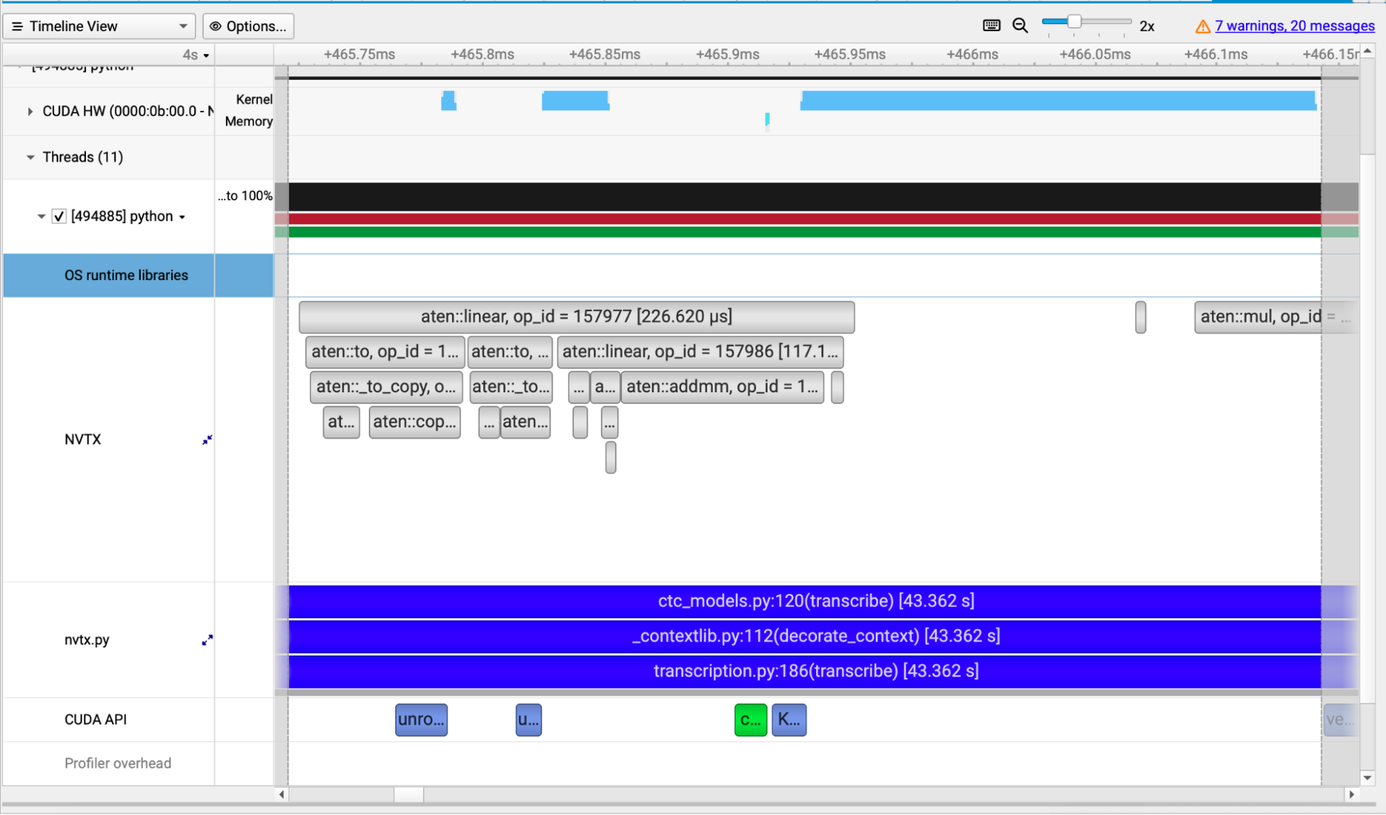
The overhead of these extra casts is significant. Figure 2 shows how casting before a matrix multiplication in the Parakeet CTC 1.1B model adds 200 microseconds of overhead, while the matrix multiplication itself only takes 200 microseconds—meaning half of the run time is spent on casting. This is captured by NVIDIA Nsight Systems, a profiling and analysis tool that visualizes workload metrics on a timeline for performance tuning.
In the CUDA HW row of Figure 2:
- The first two light blue sections indicate the kernels handling the casting from
float32tobfloat16. - The empty white regions indicate the casting overhead taking 200 microseconds of the total 400 microseconds runtime.
Resolving AMP overheads with full half-precision inference
To address challenges associated with AMP, we implemented best practices by performing inference fully in half precision (either float16 or bfloat16). This approach, described in NVIDIA/NeMo pull requests on GitHub, eliminates unnecessary casting overhead without compromising accuracy, as precision-sensitive operations like softmax and layer norm still use float32 under the hood, even when half precision inputs are specified. See the AccumulateType and SoftMax examples.
You can enable this in examples/asr/transcribe_speech.py by setting compute_dtype=float16 or compute_dtype=bfloat16 while ensuring amp=True is not set (default is amp=False). Setting both amp=True and a value for compute_dtype will cause an error. If you are writing your own Python code, simply call model.to(torch.bfloat16) or model.to(torch.float16) to achieve this optimization, as demonstrated at NeMo/examples/asr/transcribe_speech.py.
Optimizing batch processing for enhanced performance
In NeMo, certain operations were originally executed sequentially, processing one element of a mini-batch at a time. This approach caused slowdowns, as each kernel operation runs quickly at batch size 1, but the overhead of launching CUDA kernels for each element leads to inefficiencies. By switching to fully batched processing, we take full advantage of the GPU streaming multiprocessor resources.
Two specific operations, CTC greedy decoding and feature normalization, were impacted by this issue. By moving from sequential to fully batched processing, we achieved a 10% increase in throughput for each operation, resulting in an overall speedup of approximately 20%.
SpecAugment became 8-10x faster after resolving similar issues. (This runs only during training, so is not the focus here.)
Low compute intensity in RNN-T and TDT prediction networks
RNN-T and TDT models have long been seen as unsuitable for server-side GPU inference due to their autoregressive prediction and joint networks. For instance, in the Parakeet RNN-T 1.1B model, greedy decoding consumed 67% of the total runtime, even though the prediction and joint networks made up less than 1% of the model’s parameters.
The reason? These kernels perform so little work that their performance is completely bounded by the kernel launch overhead, leaving the GPU idle most of the time. To illustrate, a CUDA kernel might take only 1 to 3 microseconds to execute, while launching one can take 5 and 10 microseconds. In practice, we found the GPU was idle for about 80% of the time, indicating that eliminating this idle time we could speed up inference 5x.
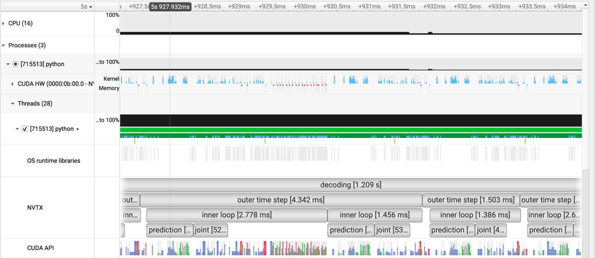
Figure 3 shows a snapshot of a few “outer time steps” of the RNN-T greedy decoding algorithm. The CUDA HW row contains multiple blank (non-blue) regions, indicating times when no CUDA code is executing. Since each outer time step in the algorithm corresponds to processing a single 80 milliseconds frame of input, running for 1.5 to 4.3 milliseconds is unacceptably slow.
In the CUDA HW row of Figure 3, regions that are not blue indicate when no CUDA code is executing (GPU is idle).
Eliminating low compute intensity with dynamic control flow in CUDA Graphs conditional nodes
Traditionally, CUDA Graphs are used to eliminate kernel launch overhead. However, they haven’t supported dynamic control flow, such as while loops, making them unsuitable for straightforward use in greedy decoding. CUDA Toolkit 12.4 introduced CUDA Graphs conditional nodes, which enable dynamic control flow.
We used these nodes to implement greedy decoding for RNN-T and TDT models, effectively eliminating all kernel launch overhead in the following files:
The latter two files implement the label-looping variant of greedy decoding, discussed in the next section.
For a detailed explanation of the problem and our solution, see our paper, Speed of Light Exact Greedy Decoding for RNN-T Speech Recognition Models on GPU. Additionally, we have submitted a pull request to PyTorch to support conditional nodes in pure PyTorch, without requiring any direct interaction with CUDA APIs, using its new torch.cond and torch.while_loop control flow APIs.
Divergence in RNN-T and TDT prediction networks
One significant issue with performing batched RNN-T and TDT inference is the divergence in vanilla greedy search algorithms. This divergence can cause some inputs to progress while others stall, leading to increased latency when using larger batch sizes. As a result, many implementations opt for inference with a batch size of 1 to avoid this issue. However, using a batch size of 1 prevents full hardware utilization, which is inefficient and uneconomical.
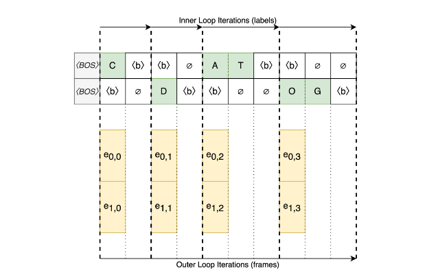
The conventional decoding algorithm (Figure 4), commonly used for transducer decoding, involves a nested-loop design:
- Outer loop: Iterates over frames (the encoder output)
- Inner loop: Retrieves labels one by one until the special blank symbol is encountered
For each non-blank symbol, both the hidden state and the output of the autoregressive prediction network should be updated. During batched inference, the inner loop can produce a varying number of labels for different utterances in the batch. Consequently, the number of calls to the prediction network is determined by the maximum number of non-blank labels across all utterances for each frame, which is suboptimal.
Figure 4 shows an example of a conventional frame-looping decoding algorithm with two utterances in a batch, four frames each, and CAT and DOG transcriptions. ∅ denotes unnecessary computations in batched decoding.
Solving divergence with efficient new decoding algorithm
To address conventional frame-looping decoding algorithm issues, we introduced a new label-looping algorithm that also uses nested loops but with a key difference: the roles of the loops are swapped (Figure 5).
- Outer loop: Iterates over labels until all frames have been decoded.
- Inner loop: Iterates over frames, identifying the next frame with a non-blank label for each utterance in the batch. This is done by advancing indices pointing to the current encoder frames, which vary for each utterance in the batch.
Figure 5 shows an example of the new label-looping decoding algorithm with two utterances in a batch, four frames each, and CAT and DOG transcriptions. ∅ denotes unnecessary computations in batched decoding.
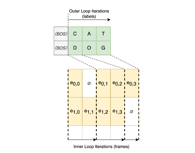
In this approach, the prediction network is evaluated at each step of the outer loop with the maximum possible batch size. The number of such evaluations is precisely the length of the longest transcription (in number of tokens) across all utterances, making it the minimum number of evaluations required. The inner loop performs operations only using the joint network. To enhance efficiency, encoder and prediction network projections are applied early in the process, minimizing the need for costly recalculations.
This batched label-looping algorithm significantly increases efficiency for both RNN-T and TDT networks, enabling much faster decoding—even when implemented with pure PyTorch code without additional GPU-specific optimization.
Performance enhancements up to 10x faster and up to 4.5x more cost-effective
The label-looping and CUDA Graphs have brought transducer models inverse real time factor i.e. RTFx (duration of audio generated / computation time; higher is better) closer than ever to that of CTC models. This impact is particularly pronounced in smaller models, where reduced kernel launch overheads—especially in operations involving small data sizes like prediction network weights and input tensors—result in even greater performance gains. Additionally, CTC models have seen substantial speed improvements thanks to the newly implemented vectorized feature normalization decoding implementations.
All these up to 10x speed enhancements (Figure 1) are available in NVIDIA NeMo ASR models with NeMo 2.0.0, which offers a fast and cost-effective alternative to CPUs.
To better illustrate benefits of ASR GPU-based inference, we estimated the cost of transcribing 1 million hours of speech using both CPUs and NVIDIA GPUs commonly available on cloud platforms like AWS, focusing on compute-optimized instances. For this comparison, we used the NVIDIA Parakeet RNN-T 1.1B model.
- CPU-based estimation: For the CPU estimation, we run NeMo ASR with batch size of 1 on a single pinned CPU core. This method, a common industry practice, allows for linear scaling across multiple cores, while maintaining a constant RTFx. We selected AMD EPYC 9454 CPU with a measured RTFx of 4.5, which is available via Amazon EC2 C7a compute-optimized instances.
- GPU-based estimation: For GPU, we used the results from the Hugging Face Open ASR Leaderboard, which were run on NVIDIA A100 80GB. The equivalent AWS instance is
p4de.24xlarge, featuring 8x NVIDIA A100 80GB GPUs. - Cost calculation: To calculate the total cost for both CPU and GPU, we:
- Divided 1 million hours of speech by the respective RTFx.
- Rounded up to the nearest hour.
- Multiplied the result by the hourly instance cost.
As shown in Table 1, switching from CPUs to GPUs for RNN-T inference yields up to 4.5x cost savings.
| CPU/GPU | AWS instance | Hourly cost | # of vCPU/GPU | Streams per instance* | RTFx (single unit) | Total RTFx | Cost of 1M hr transcription |
| AMD Epyc 4th Gen | C7a.48xlarge | $9.85 | 192 | 192 | 4.5 | 864 | $11,410 |
| NVIDIA A100 80GB | P4de.24xlarge | $40.97 | 8 | 512 | 2053 | 16425 | $2,499 |
* CPU or global batch size for GPU
Accelerate your transcriptions with NVIDIA ASR
NVIDIA NeMo boosts performance speed up to 10x across ASR models that top Hugging Face Open ASR Leaderboard. This leap in speed is powered by innovations such as autocasting tensors to bfloat16, the label-looping algorithm, and CUDA Graphs optimizations.
These accelerated performances also enable significant cost savings. For example, NeMo GPU-powered inference on the NVIDIA A100 offers up to 4.5x cost savings compared to CPU-based alternatives when transcribing one million hours of speech.
Continued efforts to optimize models like NVIDIA Canary 1B and Whisper will further reduce the cost of running attention-encoder-decoder and speech LLM-based ASR models. NVIDIA is also advancing its CUDA Graphs conditional nodes and integrating them with compiler frameworks like TorchInductor, which will provide further GPU speedups and efficiency gains. For more details, check out our pull request for support conditional nodes in PyTorch.
We’ve also released a smaller Parakeet hybrid transducer-ctc model, Parakeet TDT CTC 10M, that achieves an RTFx of ~4,300 with improved accuracy of average WER of 7.5 on HF ASR Leaderboard test sets, further extending the NeMo ASR capabilities.
Explore NVIDIA NIM for speech and translation for faster, cost-effective integration of multilingual transcriptions and translations into your production applications running in the cloud, in a data center, or on a workstation.


