Performing an exhaustive exact k-nearest neighbor (kNN) search, also known as brute-force search, is expensive, and it doesn’t scale particularly well to larger datasets. During vector search, brute-force search requires the distance to be calculated between every query vector and database vector. For the frequently used Euclidean and cosine distances, the computation task becomes equivalent to a large matrix multiplication.
Although GPUs are efficient at performing matrix multiplications, the computational cost becomes prohibitive with increasing data volumes. Yet many applications don’t require exact results and can instead trade off some accuracy for faster searches. When exact results are not needed, approximate nearest neighbor (ANN) methods can often reduce the number of distance computations that must be performed during search.
This post will focus on an approximate method that uses an simple inverted file index (IVF) approach, known as IVF-Flat. This algorithm provides simple knobs to reduce the overall search space and to trade-off accuracy for speed. In a subsequent post we will discuss an alternative ANN method IVF-PQ, which uses the same technique as IVF-Flat to reduce the search space, but also compresses the dataset using Product Quantization (PQ). This enables searching larger datasets at an increased throughput, but can further reduce accuracy.
To help you understand how to use IVF-Flat, we discuss how the algorithm works, and demonstrate the usage of both the Python and C++ APIs in cuVS. We cover setting parameters for index building and give tips on how to configure GPU-accelerated IVF-Flat search. These steps can also be followed in the example Python notebook and C++ project. Finally, we demonstrate that GPU-accelerated vector search can be an order of magnitude faster than CPU search.
The simple inverted index algorithm overview
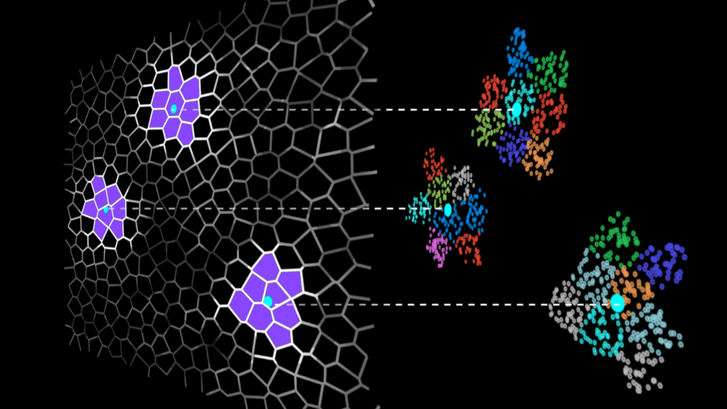
IVF methods accelerate vector search by grouping the dataset vectors into clusters and limiting the search to some number of nearest clusters for each query (Figure 1).
Searching only a few clusters (instead of the whole dataset) is the actual approximation in the IVF-Flat algorithm. Using this approximation, you might miss some neighbors that are assigned to clusters you aren’t searching, but it greatly improves search time.
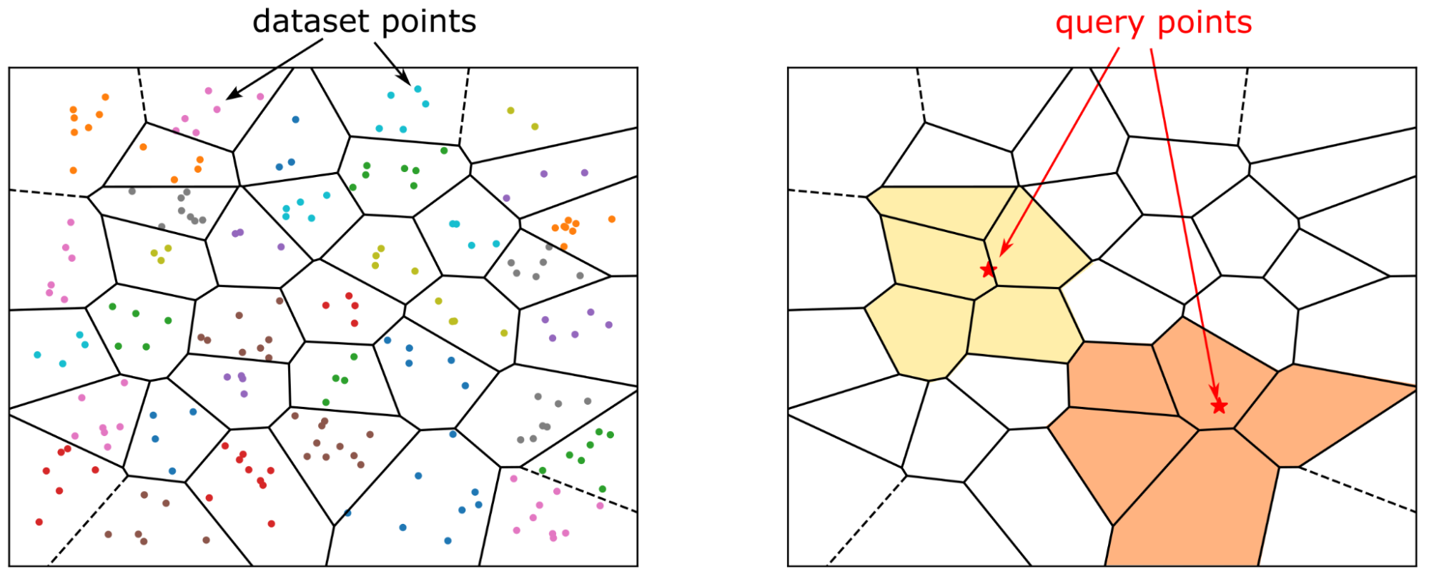
Before you can search the dataset, you must build an index, which is a structure that stores the information that you need for efficient search. For IVF-Flat, the index stores the description of the clusters: the coordinates of their center, and the list of vectors that belong to the cluster. This list is the inverted list, also known as an inverted file, and that is where the IVF acronym comes from.
In the following sections, after discussing inverted files, we demonstrate how to construct an index and explain how the search is performed.
What is an inverted index?
For completeness, here’s some historical context. The term inverted file (or inverted index) comes from the information retrieval field.
Consider a simple example of a few text documents. To search documents that contain a given word, a forward index stores a list of words for each document. You must read each document explicitly to find the relevant ones.
In contrast, an inverted index would contain a dictionary of all the words that you can search, and for each word, you have a list of document indices where the word occurs. This is the inverted list (inverted file), and it enables you to restrict the search to the selected lists.
Today, text data is often represented as vector embeddings. The IVF-Flat method defines cluster centers and these centers are analogous to the dictionary of words in the preceding example. For each cluster center, you have a list of vector indices that belong to the cluster, and search is accelerated because you only have to inspect the selected clusters.
Building an inverted index
The index building is mainly a clustering operation on the dataset. An ivf_flat index can be created in Python using the following code example:
from cuvs.neighbors import ivf_flat

build_params = ivf_flat.IndexParams(
        n_lists=1024,
        metric="sqeuclidean"
    )

index = ivf_flat.build(build_params, dataset)
In C++, you have the following syntax:
#include <raft/neighbors/ivf_flat.cuh>
using namespace cuvs::neighbors;
raft::device_resources dev_resources;

ivf_flat::index_params index_params;
index_params.n_lists = 1024;
index_params.metric = cuvs::distance::DistanceType::L2Expanded;

auto index = ivf_flat::build(dev_resources, index_params,
raft::make_const_mdspan(dataset.view()));
The most important hyperparameter for creating the index is n_lists, which tells how many clusters to use. You also specify the metric for distance calculation.
Finding the closest vectors in an inverted index
After the index is built, search is simple. In Python, the following call returns two arrays: the indices of the neighbors and their distances from the query vectors:
distances, indices = ivf_flat.search(ivf_flat.SearchParams(n_probes=50), index, queries, k=10)
The equivalent call in C++ requires preallocating the output arrays:
int topk = 10;
auto neighbors = raft::make_device_matrix<int64_t, int64_t>(dev_resources, n_queries, topk);
auto distances = raft::make_device_matrix<float, int64_t>(dev_resources, n_queries, topk);

ivf_flat::search_params search_params;
search_params.n_probes = 50;

ivf_flat::search(dev_resources,
                search_params,
                index,
                raft::make_const_mdspan(queries.view()),
                neighbors.view(),
                distances.view());
Here you search k=10 neighbors for each query. The parameter n_probes tells you how many clusters to search (or probe) for each query, and it determines the accuracy of the search.
By testing only n_probes clusters for each query, you might omit some neighbors that were assigned to clusters whose centers are farther from the query point. The quality of the search is usually measured as the recall rate, which is the fraction of the actual nearest k-neighbors out of all the returned neighbors.
Internally, the search is performed in two steps (Figure 2):
- The coarse search selects
n_probesnearby clusters for each query. - A fine search compares the query vectors to all the dataset vectors in the selected clusters.
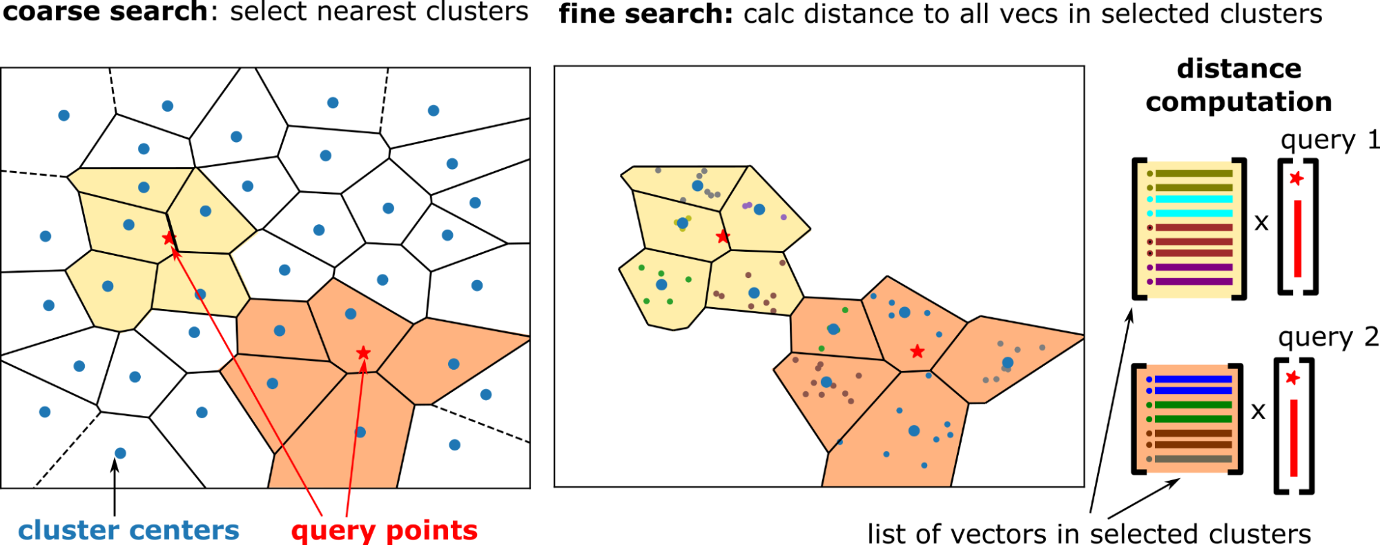
Coarse search
The coarse search is done using an exact kNN search between the cluster centers and the query vectors. Select the nearest cluster centers, n_probes clusters for each query. Coarse search is relatively cheap because the number of clusters is much smaller than the dataset size (for example, 10K clusters for 100M vectors).
Fine search
For IVF-Flat, the fine search is again an exact search. But each query has its own set of clusters to search (to probe), and the distance between the query vector and all the vectors in the probed clusters are calculated.
For small batch sizes, the regions that you search around a query point do not overlap. Therefore, the problem structure becomes a batched matrix-vector multiplication (GEMV) operation. This operation is memory bandwidth bound, and the large bandwidth of GPU memory greatly accelerates this step.
The top-k neighbors from each probed cluster are selected, which results in n_probes * k neighbor candidates for each query. This is reduced to the k-nearest neighbors.
Tuning parameters for index building
In the previous sections, you got an overview of the index building and search. Here’s a detailed look at how to set the parameters for index building.
Construction of the index consists of two phases:
- Training or computing the clusters (build): A balanced hierarchical k-means algorithm clusters the training data.
- Adding the dataset vectors to the index (extend): Dataset vectors are assigned to their cluster and added to the appropriate list of vectors in the clusters.
Number of clusters
The n_lists parameter has a profound impact on overall performance during both training and search: it defines the number of clusters into which the index data is partitioned. Setting n_lists = sqrt(n_samples) is a good starting point (where n_samples is the number of vectors in the dataset).
To make sure that the GPU resources are used efficiently, the average cluster size (that is, n_samples/n_lists) should be in the range of at least 1K vectors to keep individual streaming multiprocessors (SMs) busy.
Index building with automatic data subsampling
K-means clustering is compute-intensive. To accelerate index building, sub-sample the dataset. Using parameter kmeans_trainset_fraction=0.1 means that you use one-tenth of the dataset for training the cluster centers.
build_params = ivf_flat.IndexParams(
        n_lists=1024,
        metric="sqeuclidean",
        kmeans_trainset_fraction=0.1,
        kmeans_n_iters=20
    )
The kmeans_n_iters parameter is passed directly to the k-means algorithm during training. It’s set to a reasonable default of 20, which works for most datasets. However, this parameter is just a recommendation for the clustering algorithm. Under the hood, it usually performs more iterations in a “balancing” phase to make sure the clusters have similar sizes.
Index building with specific training data for clustering
In the previous examples, a single call to ivf_flat.build performed the clustering and added the whole dataset into the index. Alternatively, you could call ivf_flat.build to train the vectors without adding them to the index (by setting add_data_on_build=False). This allows exact control of what vectors are used for training the index. Subsequently, ivf_flat.extend can be used to add vectors to the index.
This is shown in the following Python code example:
n_train = 10000
train_set = dataset[cp.random.choice(dataset.shape[0], n_train, replace=False),:]

build_params = ivf_flat.IndexParams(
        n_lists=1024,
        metric="sqeuclidean",
        kmeans_trainset_fraction=1,
        kmeans_n_iters=20,
        add_data_on_build=False
    )

index = ivf_flat.build(build_params, train_set)
ivf_flat.extend(index, dataset, cp.arange(dataset.shape[0], dtype=cp.int64))
The dataset vectors can be added to the index by a single call to ivf_flat.extend. Internally, the data is processed batch-wise if needed to reduce memory consumption. The corresponding C++ code is as follows:
index_params.add_data_on_build = false;
// Sub sample the dataset to create trainset.
// ...
// Run k-means clustering using the training set
auto index = ivf_flat::build(dev_resources, index_params,
    raft::make_const_mdspan(trainset.view()));

// Fill the index with the dataset vectors
index = ivf_flat::extend(dev_resources,
    raft::make_const_mdspan(dataset.view()),
    std::optional<raft::device_vector_view<const int64_t, int64_t>>(),
    index);
Adding new vectors to the index
New vectors can be added at any time to the dataset by calling ivf_flat.extend. By default, the cost of growing the list of vectors is amortized away by allocating extra space when the list size is increased. C++ API users can change this behavior by setting the following parameter:
index_params.conservative_memory_allocation = true;
This can be beneficial if the number of clusters is large, and it is not expected to add vectors often.
By default, the cluster centers do not change when you add vectors to the dataset. The adaptive_centers flag can be enabled during index construction if you want the cluster centers to drift with the new data.
Tuning parameters for finding the closest vectors
Here’s how to set the parameters for search: use GPU resources efficiently and increase the value of n_probes.
GPU resources
During search, you create internal workspace memory. We recommend using a pooling allocator to reduce the overhead of memory allocation.
Constructing the RAFT resources object is time-consuming. The resources object should be reused by passing a resource handle to the search function. In Python, you can configure the device resources and the memory pool in the following way:
from cuvs.common import DeviceResources
import rmm
mr = rmm.mr.PoolMemoryResource(
     rmm.mr.CudaMemoryResource(),
     initial_pool_size=2**30
)
rmm.mr.set_current_device_resource(mr)

handle = DeviceResources()

search_params = ivf_flat.SearchParams(n_probes=50)
distances, indices = ivf_flat.search(search_params, index, queries, k=10, handle=handle)
handle.sync()
Users of the C++ API always have to pass an explicit device_resources handle, and this should be reused among separate calls to search. The pool allocator can be set up in the following way:
raft::device_resources dev_resources;
raft::resource::set_workspace_to_pool_resource(
    dev_resources, 2 * 1024 * 1024 * 1024ull);
ivf_flat::search(dev_resources, ...)
C++ users can specify a separate allocator for temporary workspace arrays, and this is used in the preceding example. The global allocator (used for creating input/output arrays) can be set using rmm::mr::set_current_device_resource.
Number of probes
The ratio n_probes/n_lists tells what fraction of the dataset is compared to each query. The number of distance computations is reduced to the n_probes/n_clusters fraction of what brute force search would compute. The quality of the search, as well as the compute time, increases as you increase n_probes, and the right value depends on the dataset.
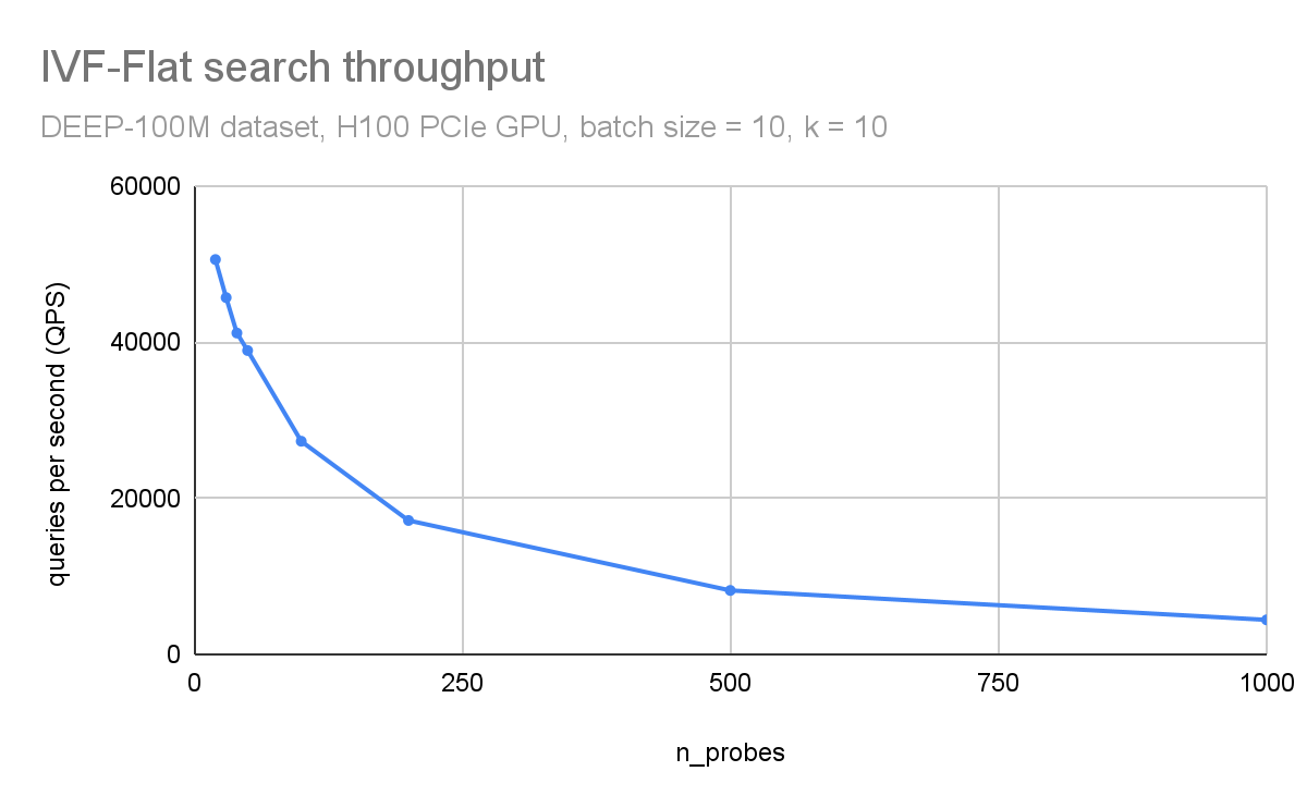
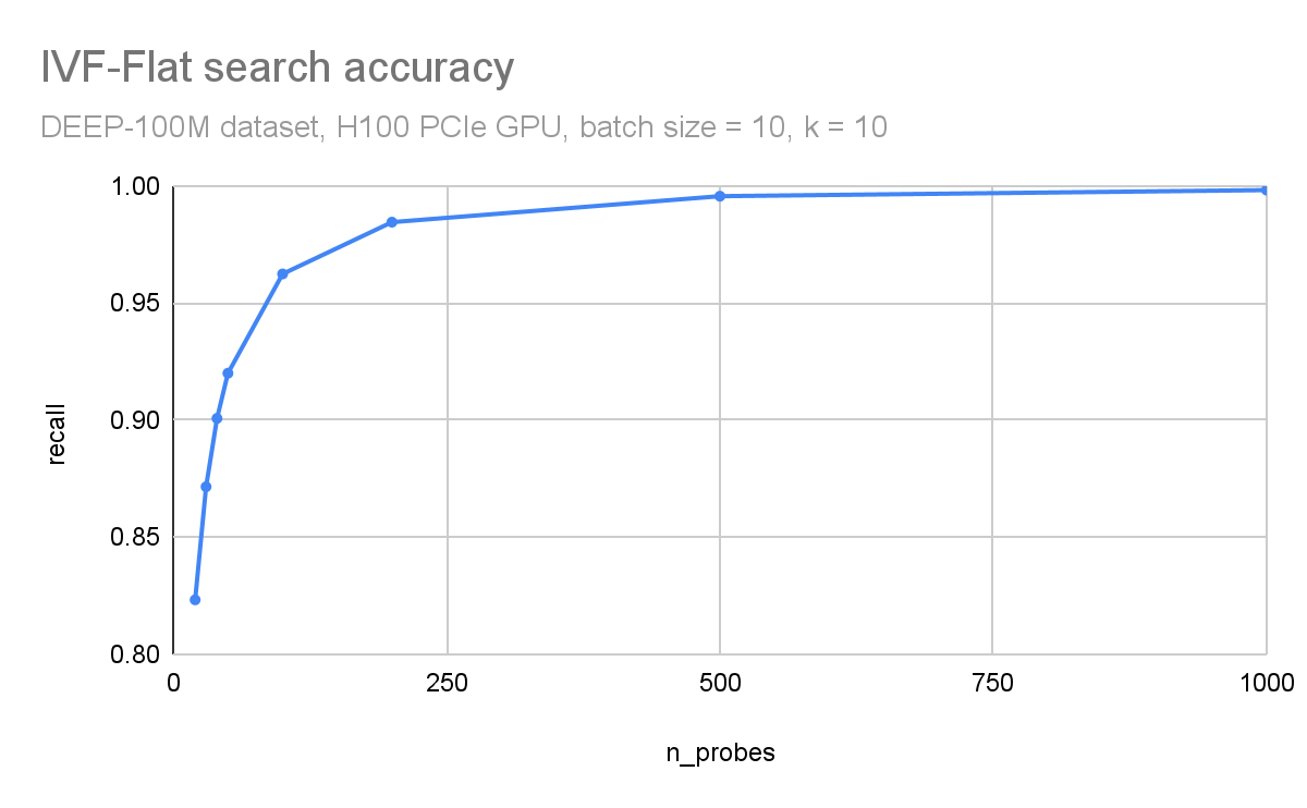
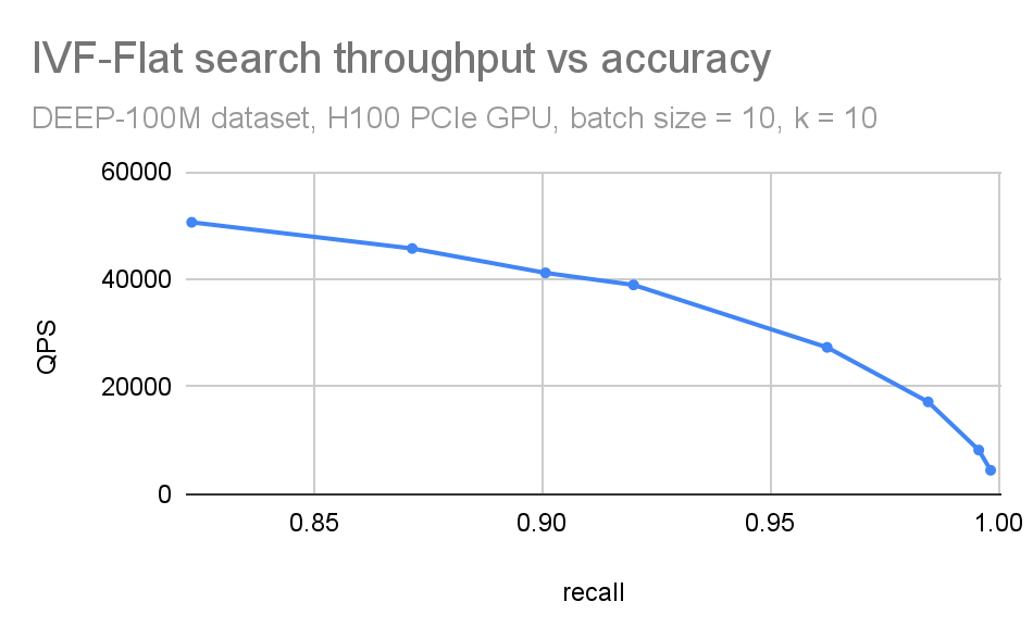
In Figure 3 and Figure 4, respectively, you can observe how throughput (queries per second) and search accuracy (recall) depends on the number of probes. Here, you are searching through 100M vectors from the DEEP1B dataset, and an H100 GPU is used for the search.
The throughput is inversely proportional to the number of probes. The dataset was divided into 100 thousand clusters. Searching just the 100 closest clusters for each query leads to a recall of 96% and searching 1000 clusters (1% of the dataset) leads to an accuracy of 99.8%.
We often combine these plots in a single QPS vs. recall plot (Figure 5). This is useful when you want to have a compact picture of the trade-off between accuracy and search throughput. It is also beneficial while comparing different ANN methods.
If n_lists == n_probes, that is like an exact (brute force) search: you compare all dataset vectors to all query vectors. You’d expect the recall to be equal to 1 in such a case (apart from small round-off errors).
As n_probes approach n_lists, IVF-Flat becomes slower than brute force because of the extra work the algorithm does (coarse plus fine search). In practice, searching around 0.1-1% of lists is enough for many datasets. But this depends on how well the input can be clustered.
Due to the surprising behavior of distance metrics in high dimensions space, clustering becomes difficult if the dataset has no structure (for example, uniform random numbers). In those cases, IVF methods don’t work well.
Performance evaluation of inverted index build time and search
The cuVS library provides a fast implementation of the IVF-Flat algorithm. Indexing 100M vectors can be done in under a minute (Figure 6). This is 14x faster than a CPU.
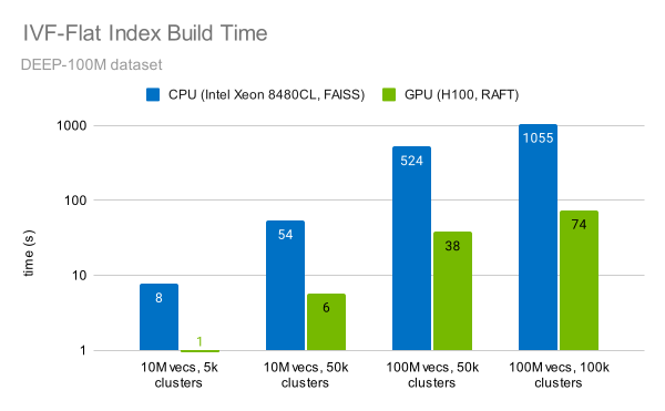
There are two main factors that enable this speedup:
- High compute throughput of the GPU: cuVS uses Tensor Cores to accelerate the k-means clustering during index building.
- The improved algorithm: RAFT uses a balanced hierarchical k-means clustering, which clusters the dataset efficiently even as the number of vectors reaches hundreds of millions.
You can also observe that the time to construct the index increases linearly with the number of vectors, and linearly with the number of clusters.
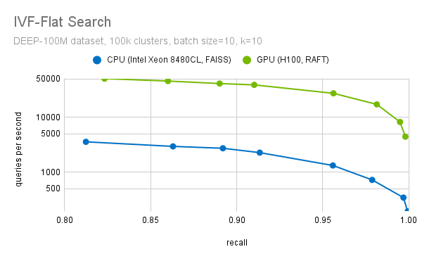
Searching through the index is facilitated by the high memory throughput of the GPU. cuVS’s IVF-Flat index uses an optimized memory layout. The vectors are interleaved for vectorized memory access to ensure large bandwidth utilization while looping through the dataset vectors in each probed cluster.
Another important step during the fine search is to filter out the top-k candidates. We have highly optimized methods to select the top-k candidates. We use optimized block-select-k kernel fused into the distance computation kernels. This enables a more than 20x speedup (at recall=0.95), when we compare the performance of cuVS IVF-Flat to a CPU implementation, as the plot in Figure 7 shows.
Summary
When performing vector search in large databases, it’s important to be aware of the high cost of an exact search, as it can result in low latency not suitable for online services.
The NVIDIA cuVS library provides efficient algorithms that improve vector search latency and throughput by focusing the search to the most relevant part of the dataset. This post discussed how the cuVS IVF-Flat algorithm works and how to set the parameters for index building and searching. Finally, we presented benchmarks to highlight the superior performance of GPUs for IVF-Flat search.
cuVS is an open-source library for vector search and more. It provides an easy-to-use C, C++,Python, and Rust APIs so you can integrate GPU-accelerated vector search into your applications. We love to hear your feedback! Send us questions and report issues on the GitHub repo. You can also find us on X (Twitter) @rapidsai.
