生成式人工智能/大语言模型

量化感知训练如何实现低精度恢复

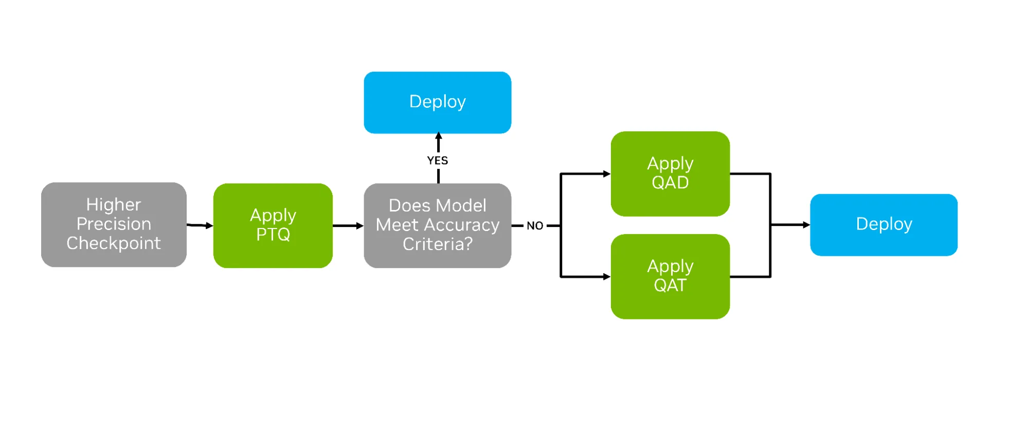
训练 AI 模型后,可采用多种压缩技术来优化模型的部署。其中较为常见的是后训练量化(PTQ),该方法通过数值缩放技术,将模型权重近似表示为低精度数据类型。然而,在 PTQ 效果有限的情况下,量化感知训练(QAT)和量化感知蒸馏(QAD)这两种替代策略则表现更优,它们通过在训练过程中主动适配低精度环境,使模型更好地适应量化部署(参见下文图 1)。

QAT 和 QAD 旨在模拟量化在后训练阶段的影响,使高精度模型的权重和激活能够适应新量化格式的可表示范围。这种适应有助于实现从高精度到低精度的平滑过渡,通常可显著提升精度恢复效果。

Flowchart showing the decision process for model quantization and deployment. It begins with a higher precision checkpoint. The model first undergoes Post-Training Quantization (PTQ). If accuracy criteria are met, the model is deployed. If not, Quantization Aware Training (QAT) or Quantization Aware Distillation (QAD) is applied. From there the model is either deployed if accuracy criteria are met, or iteratively refined.
图 1。用于 PTQ、QAT 和 QAD 的决策流程,展示模型如何根据准确性标准推进部署。

在本博客中,我们将探讨量化感知训练(QAT)和量化感知部署(QAD),并演示如何使用 TensorRT Model Optimizer 应用这两种技术。Model Optimizer 提供了与 Hugging Face 和 PyTorch 原生兼容的 API,使开发者能够在沿用熟悉训练流程的同时,无缝地为 QAT 和 QAD 准备模型。在完成模型训练后,我们还将展示如何利用 TensorRT-LLM 高效地导出并部署这些模型。

什么是量化感知训练? 

QAT 是一种在模型预训练后引入的额外训练阶段,旨在使模型能够适应低精度计算。与 PTQ 不同,PTQ 依赖校准数据集在不进行训练的情况下对已训练好的模型进行全精度量化,而 QAT 则在前向传播过程中直接使用量化值进行训练。QAT 的工作流程与 PTQ 基本相似,主要区别在于:在对原始模型应用量化方法后,会额外插入一个训练阶段(如图 2 所示)。

Flowchart illustrating the Quantization Aware Training (QAT) workflow. On the left, an original precision model is combined with calibration data and a Model Optimizer quantization recipe to form a QAT-ready model. This model, along with a subset of original training data, enters the QAT training loop. Inside the loop, high-precision weights are updated and then used as “fake quantization” weights during the forward pass. Training loss is calculated, and the backward pass uses a straight-through estimator (STE) to propagate gradients. The loop repeats until training converges.
图 2。量化感知训练 (QAT) 工作流,展示如何使用模拟的低精度权重来准备、量化和迭代训练模型。

QAT 的目标是生成高精度的量化模型,从而实现优异的推理性能。这使其与旨在提升训练效率的量化训练有所区别。因此,QAT 可能不会采用训练吞吐量最优的方法,但能够产出推理精度更高的模型。

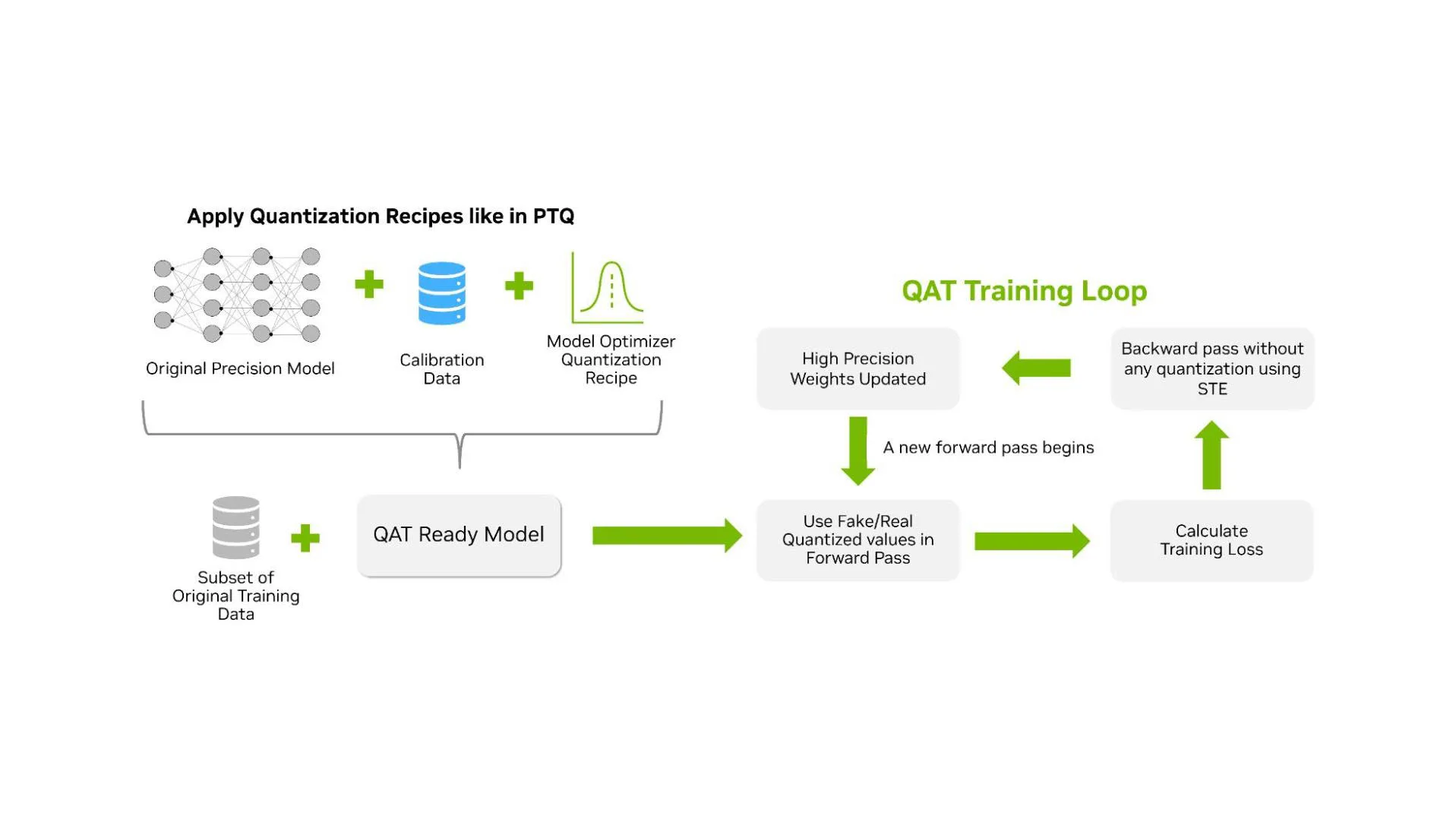
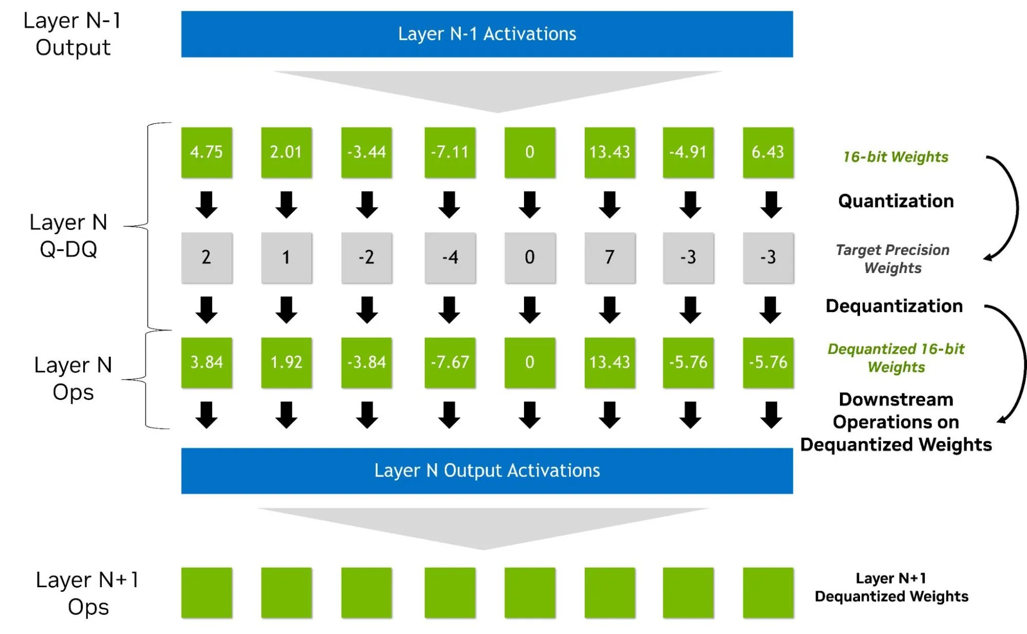
QAT 通常在前向传播过程中采用“假量化”方式处理权重和激活值。该方法通过在较高精度的数据类型中插入量化与反量化操作来模拟低精度计算(如图 3 所示),因此无需依赖原生硬件支持。例如,NVFP4 的 QAT 可在 Hopper GPU 上通过模拟量化实现。这种方法能够自然地集成到现有的高精度训练流程中:反向传播时仍以较高精度计算梯度,并将量化操作建模为透传操作(即直通估计,STE)。此外,还可引入其他优化步骤(如对异常梯度进行归零处理),但可能会带来超出 BF16 或 FP16 训练的额外开销。

通过在训练过程中将舍入和裁剪误差纳入损失函数,QAT 使模型能够适应这些误差并从中恢复。尽管在实践中 QAT 可能无法显著提升训练性能,但它提供了一种稳定且实用的训练方式,有助于生成高精度的量化推理模型。

ext Infographic showing the Quantize Dequantize workflow across two adjacent neural network layers. A blue bar at the top labeled “Layer N minus 1 Activations” narrows through a gray funnel into Layer N. Inside Layer N, three stacked rows of small squares represent the weight path: the top row is green with decimal numbers and is labeled 16 bit Weights; the middle row is gray with small integers and is labeled Target Precision Weights, indicating quantized values; the bottom row is green with decimals and is labeled Dequantized 16 bit Weights. A bracket on the left marks the top two rows as Layer N Q DQ and the bottom row as Layer N Ops, indicating that matmul and similar operations use the dequantized values. On the right, callouts read 16 bit Weights, Quantization, Target Precision Weights, Dequantization, Dequantized 16 bit Weights, and Downstream Operations on Dequantized Weights. Below, a second blue bar labeled “Layer N Output Activations” narrows to a row of green squares labeled Layer N plus 1 Ops with a note “Layer N plus 1 Dequantized Weights.” The figure communicates that quantization error is introduced at quantize, dequantize restores datatype for compatibility, shapes are unchanged, and the next layer consumes dequantized activations together with its own dequantized weights.
图 3。此图说明了在 QAT/ PTQ 期间跨相邻层的“假量化”。N 层的权重被量化为目标精度,立即去量化回 BF16/ FP16,然后由层的运算使用,因此计算基于近似 (去量化) 值运行。随后,生成的 N 层输出激活函数会馈送 N+ 1 层,该层同样使用去量化权重,这表明下一层的输入是去量化激活函数,而精度错误则源于量化并持续存在于下游。

某些 QAT/QAD 实现无需使用假量化,但这些方法不在本文讨论范围内。在当前的 Model Optimizer 实现中,QAT 的输出是一个精度保持不变的新模型,其权重已更新,并包含转换为目标格式所需的关键元数据,例如:

  • 每层激活的缩放系数 (动态范围)
  • 比特等量化参数
  • 块大小

如何使用 Model Optimizer 应用 QAT

将 QAT 与 Model Optimizer 结合使用非常简便。QAT 支持与 PTQ 工作流相同的量化格式,涵盖 FP8、NVFP4、MXFP4、INT8 和 INT4 等多种关键格式。在以下代码片段中,我们选择了 NVFP4 格式对权重和激活进行量化。

import modelopt.torch.quantization as mtq

config = mtq.NVFP4_MLP_ONLY_CFG

# Define forward loop for calibration
def forward_loop(model):
    for data in calib_set:
        model(data)

# quantize the model and prepare for QAT
model = mtq.quantize(model, config, forward_loop) 

到目前为止,代码与 PTQ 保持一致。为了应用 QAT,我们需要执行训练循环,该循环包含一系列标准的可调参数,例如优化器的选择、学习率、调度器等。

# QAT with a regular finetuning pipeline
# Adjust learning rate and training epochs
train(model, train_loader, optimizer, scheduler, ...)

为获得更佳效果,我们建议将 QAT 的运行时间设置为初始训练时长的约 10%。在大语言模型方面,我们发现,即使微调时间不足原始预训练时间的 1%,QAT 通常也足以恢复模型的性能。若希望深入了解 QAT,欢迎探索完整的 Jupyter Notebook 教程

什么是量化感知蒸馏?

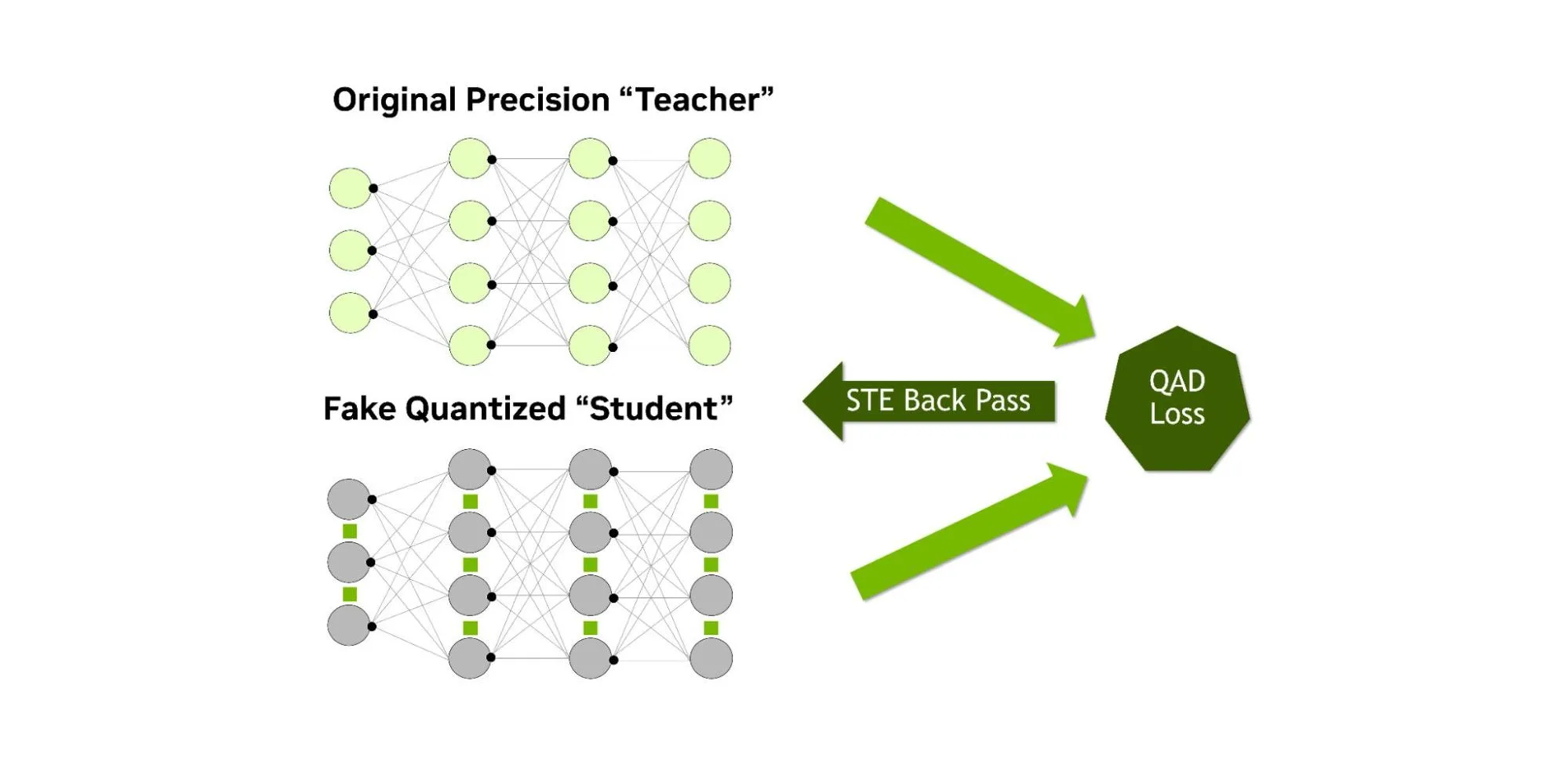
与 QAT 类似,QAD 的目标是在训练后量化过程中恢复模型的准确性,同时引入知识蒸馏机制。与传统的知识蒸馏方法(通常由较大的“教师”模型指导较小的“学生”模型)不同,在 QAD 中,“学生”模型仅在前向传播过程中引入伪量化操作。教师模型是使用相同数据训练得到的原始高精度模型。蒸馏过程通过蒸馏损失来衡量量化模型预测结果的偏差,从而使量化后“学生”模型的输出与全精度“教师”模型的输出保持一致(如图 4 所示)。

Flowchart of Quantization Aware Distillation (QAD). On the left, an original precision model is combined with calibration data and a quantization recipe to create a QAD-ready student model. This student model is paired with a higher precision teacher model and a subset of the original training data. In the QAD training loop, the student uses “fake quantization” weights in its forward pass, while the teacher performs a standard forward pass. Outputs are compared to calculate QAD loss, which combines distillation loss with standard training loss. Gradients flow back through the student model using a straight-through estimator (STE), and the student’s high-precision weights are updated to adapt to quantization conditions.
图 4。QAD 在教师指导下训练低精度学生模型,将蒸馏损失与标准 QAT 更新相结合。

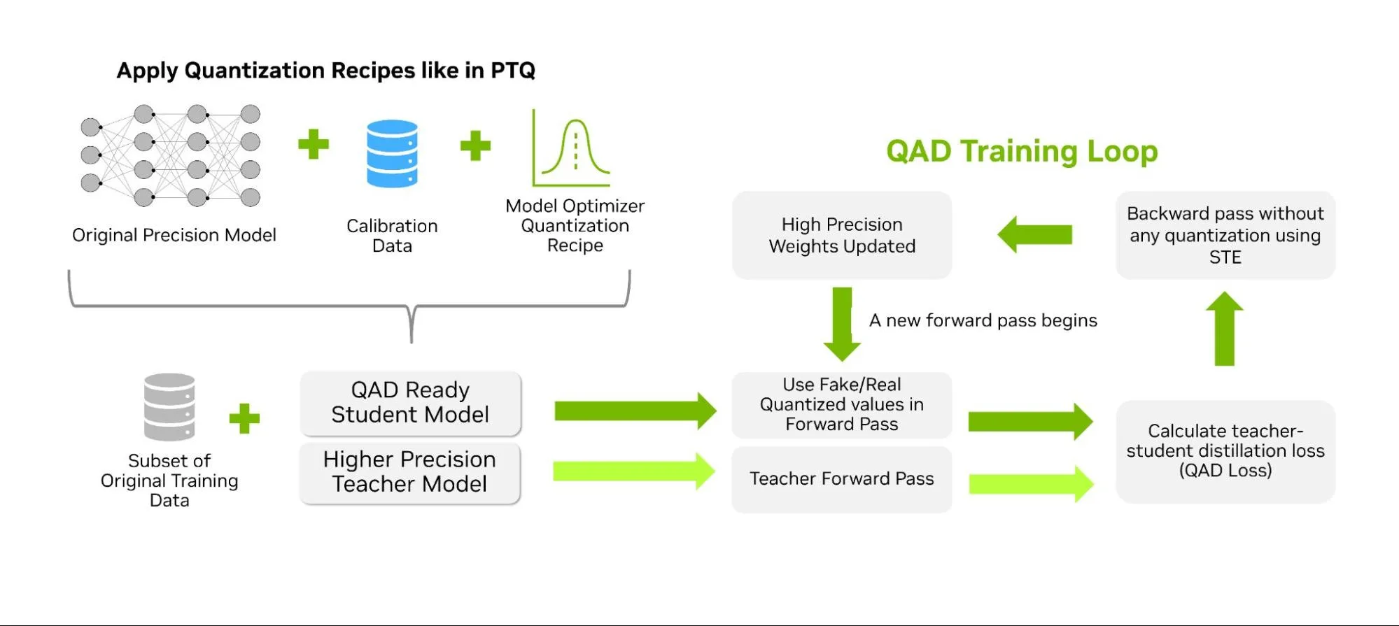
在蒸馏过程中,学生的计算采用假量化方式,而教师模型则保持全精度。由于量化引入的任何偏差都会直接反映在蒸馏损失中,低精度的权重和激活函数便能依据教师模型的行为进行调整(如图5所示)。经过QAD处理后,所得模型在推理性能上与PTQ和QAT方法相当(因为精度和架构均未改变),但由于蒸馏损失提供了额外的学习信号,准确率的恢复可能更为显著。

Diagram of the gradient and loss flow in Quantization Aware Distillation (QAD). On the left, a loss landscape curve illustrates gradient descent, with a note that high precision math is used for gradient computation and weight accumulation. In the center, a neural network represents the student model: original precision weights are updated under quantization conditions. A green arrow labeled “Straight Through Estimator” carries gradients backward. On the right, the student’s outputs are compared to the teacher’s outputs to calculate distillation loss, which is combined with standard QAT loss to form the overall QAD loss.
图 5。QAD 损失将教师的蒸馏损失与 QAT 损失相结合,在量化条件下通过 STE 更新学生权重。

在实践中,这种方法比先提炼FP32模型再进行量化更为有效,因为QAD流程能够更好地兼顾量化误差,并直接对模型进行相应调整。

如何使用 Model Optimizer 应用 QAD

TensorRT Model Optimizer 目前提供了用于实现该技术的实验性 API。该流程与量化感知训练(QAT)和后训练量化(PTQ)类似,首先需将量化方法应用于学生模型。随后,可配置知识蒸馏的相关参数,包括指定教师模型、训练参数以及蒸馏损失函数等。QAD API 将持续优化,以进一步简化该技术的应用流程。如需获取最新的代码示例和文档,可访问 Model Optimizer 代码仓库中的 QAD 模块

评估 QAT 和 QAD 的影响

并非所有模型都需要进行 QAT 或 QAD——在仅采用 PTQ 的关键基准测试中,许多模型的原始准确率仍能保持在 99.5% 以上。

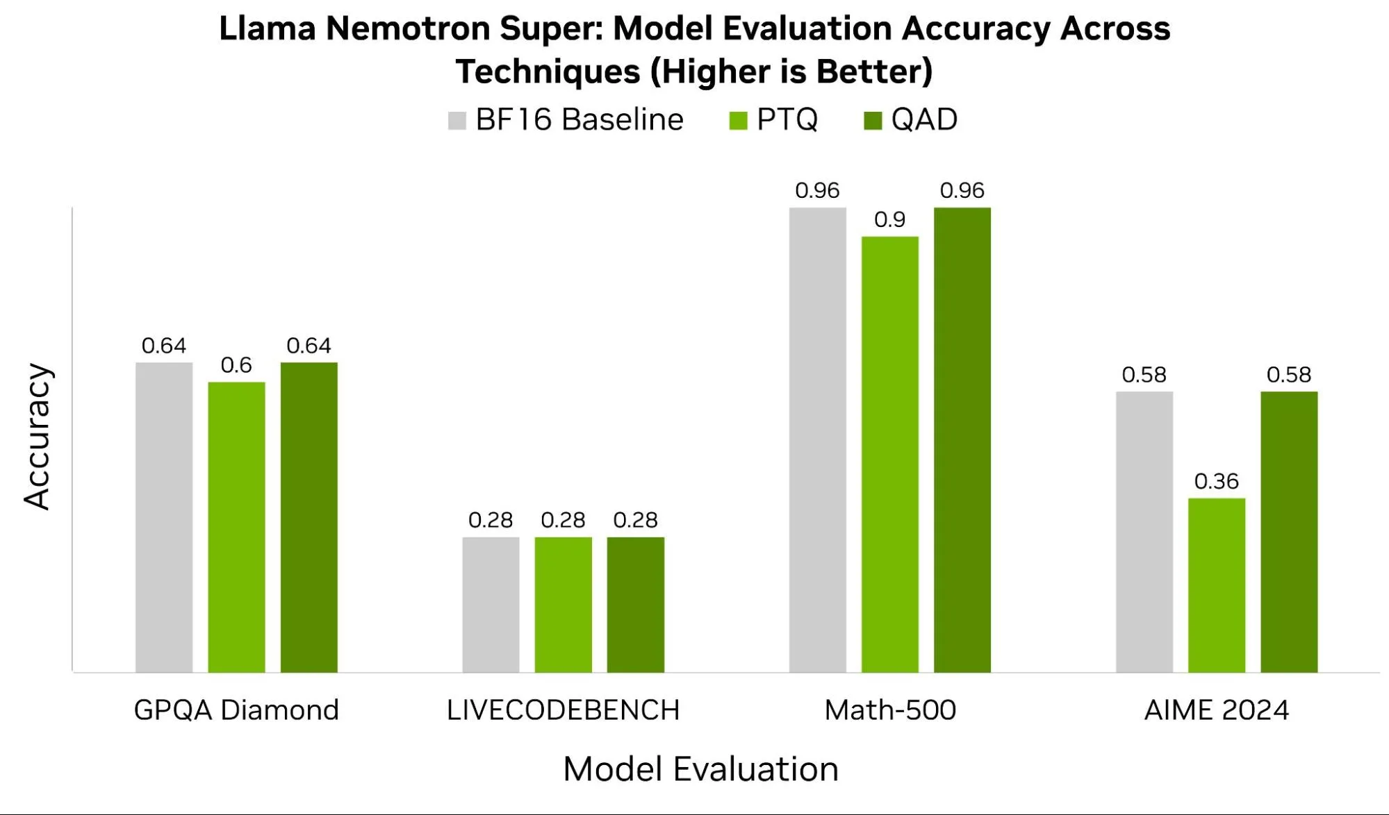
在某些情况下,例如 Llama Nemotron Super 模型,我们观察到 QAD 具有显著优势。图 6 展示了该模型在 GPQA Diamond、LIVECODEBENCH、Math-500 和 AIME 2024 等基准测试上的表现,对比了采用 BF16 精度的原始模型与经过 PTQ 和 QAD 量化后的检查点结果。除 LIVECODEBENCH 外,其他所有基准测试均显示,QAD 能够恢复 4% 至 22% 的准确率损失。

Bar chart comparing model evaluation accuracy across quantization techniques for the “Super Llama Nemotron Reasoning” model. The chart measures accuracy for four benchmarks: GPQA Diamond, LIVECODEBENCH, Math-500, and AIME 2024. For GPQA Diamond, BF16 baseline scores 0.64, PTQ 0.60, and QAD 0.64. LIVECODEBENCH shows equal accuracy of 0.28 for BF16, PTQ, QAT, and QAD. On Math-500, BF16 baseline achieves 0.96, PTQ 0.90, QAT 0.96, and QAD 0.96. For AIME 2024, BF16 baseline scores 0.58, PTQ 0.36, QAT 0.58, and QAD 0.58. Overall, QAD consistently matches BF16 accuracy while PTQ lags behind in some benchmarks.
图 6。QAD 使用 Super Llama Nemotron 推理在基准测试中保持基准准确性,在 Math-500 和 AIME 2024 等任务中的表现优于 PTQ。此模型未测量 QAT 准确度,但预计可在 PTQ 和 QAD 之间进行评分。

在实践中,QAT 和 QAD 的效果在很大程度上依赖于训练数据的质量、超参数的选择以及模型架构的设计。在对 4 位数据类型进行量化时,NVFP4 等格式能够从更精细、更精确的扩展因子中获益。

下图7展示了Llama-Nemotron Nano在NVFP4和MXFP4格式下于常见VLM基准测试中的准确率表现。在OpenVLM Hugging Face Leaderboard中,AI2D、ChartQA和DocVQA等基准测试中,NVFP4的得分 consistently 超出MXFP4超过1%。尽管这一差异看似微小,但在实际应用中可能带来显著影响。参考排行榜可见,在特定基准测试中,领先模型与后续模型之间的性能差距通常仅为几个百分点。

ar chart titled “Llama-Nemotron Nano VLM – Model Evaluation Accuracy MXFP4 and NVFP4 (Higher is Better).” The x axis is Model Evaluation with five tasks: AI2D, ChartQA, InfoVQA, OCRBench, and DocVQA. The y axis is Accuracy. Each task shows two bars: light gray labeled MXFP4 QAD and green labeled NVFP4 QAD. Numeric labels above bars read approximately: AI2D 98.58 and 98.70, ChartQA 98.84 and 98.96, InfoVQA 95.60 and 99.07, OCRBench 99.88 and 100.00, DocVQA 99.56 and 99.89. NVFP4 QAD bars are equal to or higher than MXFP4 QAD across all tasks, with the largest gap on InfoVQA.
图 7。NVFP4 和 MXFP4 格式的 QAD 4 位精度模型评估精度与原始精度的比较。

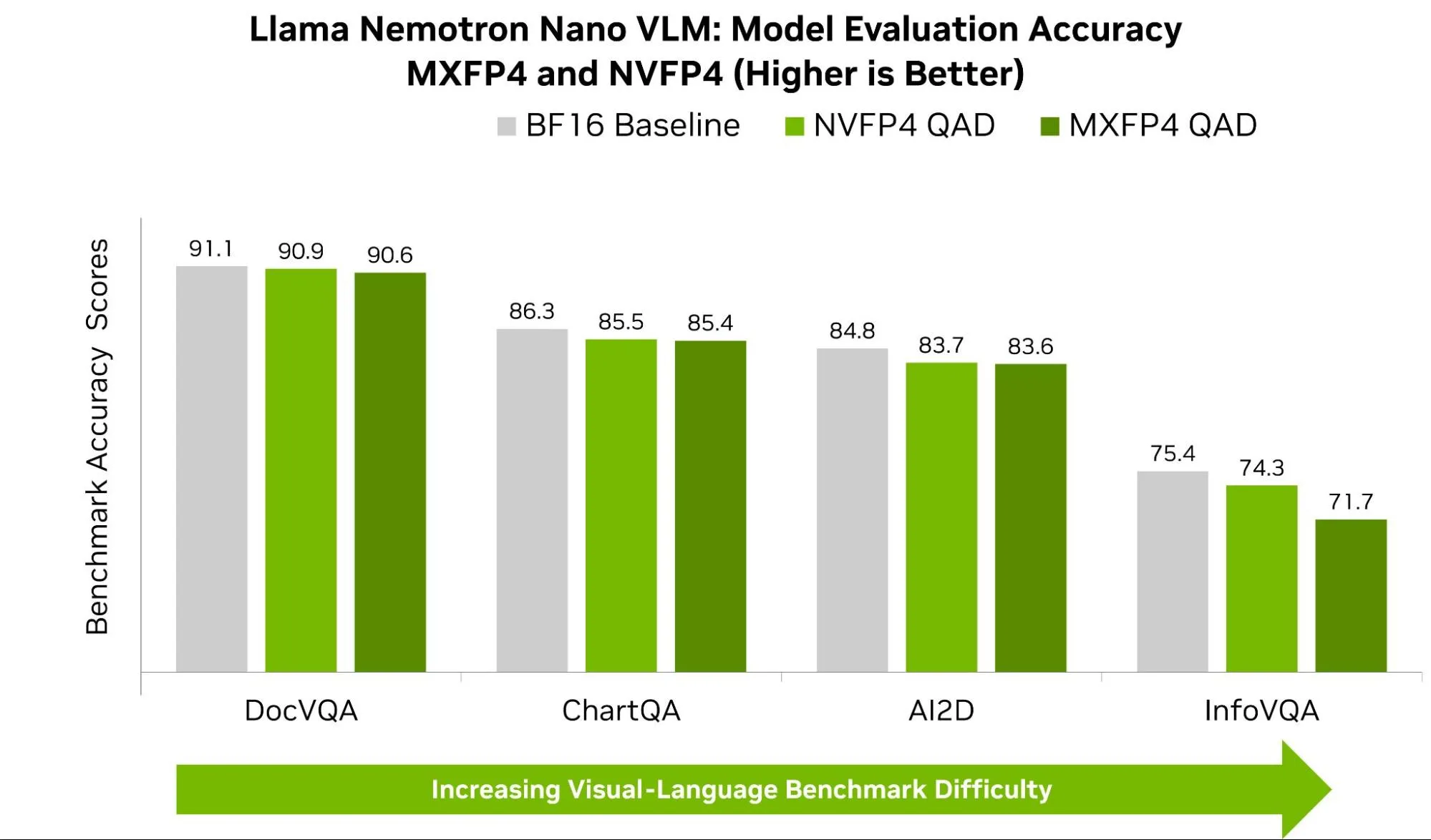
观察到在视觉问答(VQA)任务中,不同数据集之间的表现差距更为明显,例如 InfoVQA 和 DocVQA。尽管两者都涉及对图像内容的提问,但在推理过程中关注的重点有所不同。InfoVQA 的数据集通常包含复杂的图表和精细的图形,其中含有微小的数值、细线条以及细致的注释。当模型被量化至 4 位时,其捕捉这些细微视觉特征的能力可能下降。NVFP4 在这方面表现出优势,它采用更细粒度的缩放机制(更小的分块和更高精度的缩放系数),能够更有效地保留微弱信号和偶发的异常值,从而在模型的视觉与文本组件之间实现更稳定的对齐,减少因舍入或截断带来的误差。

相比之下,DocVQA 主要针对简洁且结构化的文档(如表格、发票、收据等),在定位到正确字段后,答案通常一目了然,因此两种格式的表现均已接近上限,差距也依然较小。

总结

量化感知训练(QAT)和量化感知蒸馏(QAD)使模型能够直接适应低精度环境,可在简单校准无法满足精度要求的情况下有效恢复性能,从而进一步拓展了PTQ的优势。如Math-500和AIME 2024等基准测试所示,这些技术显著缩小了低精度推理与全精度模型之间的精度差距,为开发者提供了兼具高效性与准确性的解决方案:既享有FP4级别推理的执行效率,又保留了高精度训练带来的模型鲁棒性。值得注意的是,数据集的选择以及训练超参数的设置对这些技术的效果具有重要影响,需谨慎考量。

借助 TensorRT Model Optimizer,您可以利用熟悉的 PyTorch 和 Hugging Face API,轻松尝试 NVFP4 和 MXFP4 等先进格式。无论需要 PTQ 的高效速度、QAT 的灵活性,还是 QAD 带来的精度提升,都能通过完整的工具链在 NVIDIA GPU 上实现模型的压缩、微调与部署。帮助您构建更快速、更轻量且精度更高的 AI 模型,为大规模生产做好准备。

如需深入了解,欢迎查看我们的 Jupyter Notebook 教程.


标签