
GPU Gems 3
GPU Gems 3 is now available for free online!
The CD content, including demos and content, is available on the web and for download.
You can also subscribe to our Developer News Feed to get notifications of new material on the site.
Chapter 6. GPU-Generated Procedural Wind Animations for Trees
Renaldas Zioma
Electronic Arts/Digital Illusions CE
In this chapter we describe a procedural method of synthesizing believable motion for trees affected by a wind field. The main goal of this approach is to enable the simulation and visualization of large open environments with massive amounts of vegetation. By introducing procedural animation calculations inside the vertex shader, this method works well with instancing and leverages the power of the GPU.
6.1 Introduction
Wind is an important element in creating believable and visually pleasant vegetation. The problem of simulating tree motion in a wind field is a complex, scientific topic. Most scientific approaches use physical simulation techniques based on motion equations that apply wind force to individual branches. Such simulations usually are prohibitive for time-constrained applications, and moreover, they can result in a less-than-natural look because of the inherent complexity of the underlying problem.
The actual motion of trees in a wind field depends on various factors, such as the stiffness and length of branches, the size and shape of leaf crowns, the conditions of the wind field, and turbulence inside the tree crown, as noted by Harker 2002.
Given the complexity of the forces affecting trees in the wind and actual observations of trees under natural conditions, we can observe that tree movements are random. Thus, a number of methods abandon physically correct simulations, instead modeling tree movement as a stochastic process.
6.2 Procedural Animations on the GPU
Given the large number of plants necessary to visualize natural environments, we need an efficient method for both simulating and rendering vegetation. And at the current rate of graphics hardware evolution, end users have come to expect simulated vegetation to be increasingly complex. The goals of our approach are (1) to offload motion simulation of trees from the CPU to the GPU, (2) to leverage hardware instancing to reduce the number of render calls, and (3) to allow seamless integration with GPU-based fluid simulation for an evolving wind field (Harris 2004).
6.3 A Phenomenological Approach
Physically correct simulation of tree motion is very complicated, and computational costs are too high for real-time applications. Instead, we choose to concentrate on a visual aspect of simulation. As Stam (1997) observed, motions of trees in a wind field are chaotic in nature. Thus, we can approximate complicated underlying dynamics using noise or a series of periodic functions. This observation forms the basis of our method. To increase the realism of existing approaches, we selected distinguishable visual phenomena and captured them into a set of simple rules. The final dynamics of the tree are synthesized by combining noise functions according to a set of those rules.
6.3.1 The Wind Field
In order to simplify the calculations, we define wind as a two-dimensional force field over terrain. The aerodynamics-based method for simulation of objects in fluid flows, presented in Wejchert 1991, defines the representation of force fields. Such fields define the direction and velocity of the fluid. Another commonly used name for such fields is vector fields.
A vector field can be stored as a sparse data structure. Global wind direction and velocity can be stored along with sparsely placed wind primitives, as in Di Giacomo 2001, or small vector grids to add details in the wind field—capturing phenomena caused by explosions or the rotors of a low-flying chopper, for example. A wind primitive is defined as an analytical function:
|
v = G(x, t), |
where x is the two-dimensional vector representing position inside the wind primitive, and v is a wind vector at the given position. Time t represents wind evolution over time. A wind primitive allows us to calculate wind direction and velocity for each given point inside the field, for example, repulsion or vorticity.
6.3.2 The Conceptual Structure of a Tree
Conceptually, a tree consists of a main trunk, branches, and leaves. Such a structure can be represented as a simplified hierarchy of interconnected rigid segments with the trunk as the root of the hierarchy. Each branch is represented as a single rigid segment and can rotate around the joint that connects to its parent branch. Although branches of a real tree are not rigid and can bend, we do not represent branches with several segments as a number of other methods do (such as Kanda 2003). Instead, this property is left to the rendering, where it is applied as a purely visual effect.
A shallow hierarchy, two to three nodes deep, is usually enough to represent visually plausible tree motion. An example of a hierarchy representing a tree with branches is shown in Figure 6-1. Later in the chapter we present a framework for generating animation by modeling angular motion at the joints of the hierarchy.
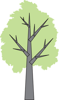
Figure 6-1 Tree Structure Represented by a Hierarchy Three Nodes Deep
For performance reasons, we omit the direct effect of leaves and small branches on the overall motion of the tree. However, such effects can be implicitly incorporated in the stochastic simulation.
We assume that the tree is initially in a state of equilibrium. Internal or constraint forces of the tree, such as branch elasticity force, are compensated for by gravity. Offline tools or modeling packages can provide solutions for these constraints.
6.3.3 The Two Categories of Simulation
Simulation levels of detail (SLODs) in animation are analogous to geometric levels of detail. Complex simulation in the distance can be replaced with a simplified version with minimal visual error. The motion of the tree trunk is the most important visual cue in the distance; in close proximity, the natural motion of the branches becomes more important. We choose to distinguish trunk and branches as two important simulation categories. Both categories benefit from the same stochastic simulation approach; however, each has its own implementation details.
Transitions between different SLODs exhibit visual popping; however, such side effects are partially concealed because of the chaotic nature of the small branch motion and the amorphous shape of the leaf crown itself.
Animating the Trunk
Trunk motion is mainly a result of the drag forces applied to the branches. In this chapter, we use drag force in terms of aerodynamics: a sum of external forces affecting a solid body in the direction of the flow. To simulate the dynamic motion of the trunk, we need to simulate the drag forces on each contributing branch and in turn propagated down the hierarchy toward the trunk.
However, it is hard to parallelize such an approach, because it would require finishing all branch simulations before the trunk could be processed. Thus, this approach would not suit implementation on the GPU. So we choose the opposite approach. We observe that the sum of all forces propagated from the branches to the trunk will result in a chaotic trunk motion. Thus, we omit the direct physical effects of the branches and instead implicitly include them in the noise function representing the motion of the trunk as a higher frequency noise.
Along with the main drag force, there are a number of other important phenomena affecting the look of the trunk motion. First, inertia resulting from the tree mass and the stiffness of the trunk will affect the amplitude and behavior of the motion. Second, because of the uneven distribution of branches, trunk motion will exhibit some movement perpendicular to wind direction along with a small amount of rotation along the axis of the trunk. And finally, turbulence in the wind field is very important, to avoid producing unnaturally synchronous movement in the tree clusters.
For performance reasons, we would like to combine all of these forces and simulate them as a single stochastic process. Luckily, there is a strong relation between external forces, the physical properties of wood, and the resulting motion of the branch (Ota 2003):
|
m a(t) + c v(t) + k x(t) = f(t), |
where m is mass, and c and k are damping and stiffness coefficients, respectively. The force f accounts for an external load due to wind. Vectors a, v, and x represent the resulting linear acceleration, linear velocity, and position of the branch, respectively.
Such a strong relation allows us to approximate underlying dynamics and synthesize motion directly. Instead of explicitly solving the dynamical equation, we directly combine the motion resulting function by carefully picking and superimposing frequency bands. An example of such a noise function, composed from the series of waves, is presented in Figure 6-2.
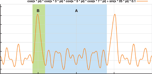
Figure 6-2 The Noise Function Used for Animating a Tree Trunk
In Figure 6-2, segment A represents a tree leaning away from the strong wind. Segment B represents the combined effect of turbulence: a temporary decrease in the wind drag force leads to a strong response by the trunk due to internal elastic (spring) force. In other words, the tree springs back and "overshoots" its point of equilibrium. Higher frequency noise adds chaotic details, simulating the effect of the smaller branches.
We can simulate a tree with greater mass and lower elasticity by lowering the amplitude of the function and decreasing the frequency. Figure 6-3 shows an example of such a function.
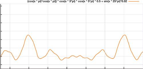
Figure 6-3 The Noise Function Used for Animating the Trunk of a Large, Stiff Tree
The final animation of the trunk results from the combination of two noise functions, representing motion parallel and perpendicular to the wind direction. An additional third noise function can be used to simulate a slight rotation around the trunk axis. As we already noted, the amplitudes of the perpendicular motion and the rotation are much lower compared with that of the parallel motion. Thus, much simpler noise functions can be used to simulate such motions while retaining the same visual quality.
Animating the Branches
Numerous methods of simulating tree motion suggest modeling the wind effect on the branches as pure drag force. However, such an approach does not completely suit trees with relatively broad, flat leaves on stiff petioles, or evergreens with thick needles. We observe that branches of such trees exhibit more aerodynamic properties, and we suggest analyzing them as wings in the wind field. Such branches will produce a lift while being affected by the wind field. Lift in terms of aerodynamics is defined as the sum of all external forces on a body acting perpendicular to the direction of the flow.
Again, we do not calculate drag and lift forces for branches explicitly. Instead, we choose to approximate the behavior of the branch with a set of simple rules, keeping in mind how drag and lift forces would affect winglike objects with single-point constraints (such as branches connected to a trunk or to another branch).
We can distinguish three different cases of spatial relation between a branch and the main trunk:
- The branch is on the wind-facing side of the tree.
- The branch is on the opposite side of the tree.
- The branch is perpendicular to the wind direction.
If the branch is facing the wind, as depicted in Figure 6-4, the combination of lift and drag forces will press it toward the trunk, and thus the branch will exhibit less free swaying. For a branch on the back side of the tree, turbulence inside the tree and the lift force will dominate over the motion of the branch, as shown in Figure 6-5. Such a branch will exhibit high-amplitude motion, such as random swaying or flapping. Finally, for a branch perpendicular to wind direction, the strong drag force and the large attack angle will cause it to bend around the axis of the parent branch. Also, the lift force will twist it a little bit around its own main axis, as shown in Figure 6-6.
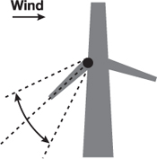
Figure 6-4 A Branch Facing the Wind
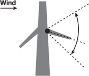
Figure 6-5 A Branch on the Back Side of the Trunk
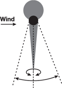
Figure 6-6 A Branch Perpendicular to the Wind Direction
Even a simple periodic function results in a visually pleasant behavior of the branch once combined according to the previous rules. The actual motion simulation for a branch will be a weighted sum of the simulated cases. Because all cases are represented as periodic functions, there is no need to explicitly solve for branch suppression, bending, and twisting constraints. Such constraints are modeled as amplitude modifiers for periodic functions.
Because the resulting motion is a weighted sum of the described cases, shearing may appear on some branches. However, such a side effect is not visually unpleasant and can be neglected.
Improvements for Branch Animations
At this point, a monotonic wind field should produce convincing tree motion overall. However, branches might move in an unnatural, synchronous way. We choose to add some variations by introducing phase shifts to the previous functions representing branch motions. A phase shift value is assigned randomly for each branch as a preprocess step. A low correlation ratio among the phase shift values will lead to very chaotic tree branch behavior, and vice versa.
Inertia is another important visual property of the branch motion. We propose to simulate the effect of inertia by using information from the trunk simulation step to modify previously discussed suppression and bending constraints (or rather, representative amplitudes). The desired visual effect is that the branches pressed toward the trunk will be released while the tree swings in the direction opposite from the wind. Such and effect creates a notion of inertia.
If accurate stiffness parameters are required per branch, the following formula mentioned in Ota 2003 can be used to modify the amplitudes of parametric motions:

where E is an elastic modulus specific to each tree species and b, t, and l are the width, thickness, and length of the branch, respectively.
6.4 The Simulation Step
The proposed stochastic approach to animation of a tree can be done completely on the GPU. Our approach has the advantage of a simulation that doesn't require information from previous iterations; thus, all branches can be processed simultaneously, independent of their position in the hierarchy. Wind field state, bone hierarchy, and tree parameters are the only required input for each step of the simulation. Required parametric functions can be combined directly on the GPU by summing series of simple periodic functions (such as cosine and sine) or can be precomputed on the CPU and passed on to the GPU as an array of samples.
The wind field can either be sampled from a two-dimensional texture in the vertex shader or be retrieved as vectors representing wind direction and velocity from the additional vertex buffer as tree-instance-specific data (using D3DSTREAMSOURCE_INDEXEDDATA in DirectX 9). The first approach is most suitable when the wind field is simulated completely on the GPU as well. Other required input data, such as bone hierarchy, noiserelated data, and miscellaneous tree parameters can be uploaded to the GPU as vertex shader constants.
The following data is associated with each branch and uploaded to the GPU in an array of vertex constants:
- The origin of the branch: the defining point around which the branch will rotate
- The main axis of the branch
- The tangent perpendicular to both the main axis of the given branch and that of its parent
- The stiffness factor of the branch
- The index specifying parent branch, or the terminating index, in case of a trunk
Along with the usual geometric information, each vertex also stores the following:
- A list of branch indices affecting a given vertex (starting from the branch to which the given vertex directly belongs and listing all parent branches until the root of the hierarchy is reached)
- A list of branch weights affecting a given vertex
The simulation step is executed for each vertex and is implemented as a part of custom vertex shader.
The list of branches affecting a given vertex is traversed during every simulation step. The list of branches is assigned for every vertex and includes branches starting from the one to which the given vertex directly to and listing all its parent branches until the root of the hierarchy is reached. Affecting branches are determined beforehand and are stored in the vertex attributes as an array of indices, as shown in Figure 6-7.
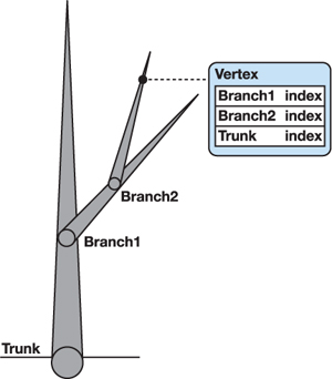
Figure 6-7 The List of Branch Indices Affecting the Given Vertex, Stored in the Vertex Attributes
For each branch affecting the given vertex, a rotation angle around its axis is calculated by combining periodic functions according to the scenarios described earlier in the chapter. Branch rotation angles are converted into a quaternion representation, as shown in Figure 6-8. Final rotation is obtained by concatenating all rotational quaternions of traversed branches for a given vertex.
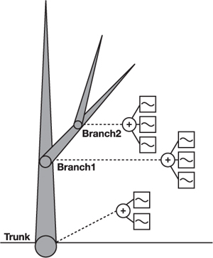
Figure 6-8 Angular Motion Is Synthesized for Each Branch
Our approach differs from conventional matrix-palette skinning (NVIDIA 2004) in two major ways: (1) we synthesize transformation matrices directly in the vertex shader, and (2) we use a concatenation operation, not linear interpolation, to obtain the final transformation. Listing 6-1 contains sample code implementing part of our method.
6.4.1 The Quaternion Library in HLSL
We chose quaternions for the simulation step implementation because they are convenient, compact, and fast while dealing with angular rotations. However, rotating vectors using a rotational matrix proved to be much faster in practice. Thus, our implementation uses quaternions only during synthesis of angular motion and then converts the result to a rotational matrix.
The following quaternion-related functions were implemented in HLSL to be used with the simulation step:
- Angle-axis-to-quaternion rotation conversions
- Quaternion concatenation
- Quaternion-to-rotation matrix conversion (Watt and Watt 1992)
Example 6-1. An HLSL Function That Simulates a Bending Branch
float4 bendBranch(float3 pos, float3 branchOrigin, float3 branchUp,
                  float branchNoise, float3 windDir, float windPower)
{
  float3 posInBranchSpace = pos - branchOrigin.xyz;
  float towardsX =
      dot(normalize(float3(posInBranchSpace.x, 0, posInBranchSpace.z)),
          float3(1, 0, 0));
  float facingWind = dot(
      normalize(float3(posInBranchSpace.x, 0, posInBranchSpace.z)), windDir);
  float a =
      branchSwayPowerA * cos(time + branchNoise * branchMovementRandomization);
  float b = branchSwayPowerB *
            cos(timeWithDelay + branchNoise * branchMovementRandomization);
  float oldA = a;
  a = -0.5 * a + branchSuppressPower * branchSwayPowerA;
  b *= windPower;
  a = lerp(oldA * windPower, a * windPower,
           delayedWindPower * saturate(1 - facingWind));
  float3 windTangent = float3(-windDir.z, windDir.y, windDir.x);
  float4 rotation1 = quatAxisAngle(windTangent, a);
  float4 rotation2 = quatAroundY(b);
  return lerp(rotation1, rotation2, 1 - abs(facingWind));
}
HLSL source code containing the necessary quaternion operations can be found on this book's DVD.
6.5 Rendering the Tree
The motion composition step uses rigid segments to represent branches. We chose to blend between two bones to conceal the resulting unnatural visual stiffness of the tree during rendering. Thus, each vertex of the tree is affected by two transformations:
- The position and rotation of the branch to which the vertex belongs
- The position and rotation of the branch one step higher in the hierarchy
Identity is used as a second transformation in case the branch is the trunk, because it is the root of the hierarchy.
For each vertex, a weighted transformation is applied to its position and normal. The vertex's tangent and binormal, if present, should be transformed analogously. The ratio of influence between the local and parent branches can be determined offline and stored in the vertex data or can be calculated at runtime as a function of distance between the vertex position and the origin of the branch, modified according to the branch stiffness parameter.
To achieve the best rendering performance, geometric level of detail should be combined with the previously discussed simulation level of detail.
6.5.1 DirectX 10
Implementation of the approach presented here has unnecessary overhead under DirectX 9, as shown in Figure 6-9: the branch transformation must be recalculated for each vertex. DirectX 10's stream-out functionality enables us to store temporary results from the simulation step and reapply them during the rendering step, as depicted in Figure 6-10, thus saving a number of operations per vertex.
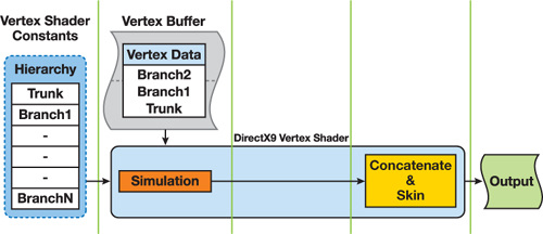
Figure 6-9 GPU Processes Under DirectX 9
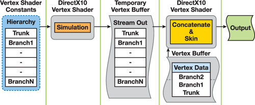
Figure 6-10 GPU Processes Under DirectX 10
DirectX 10 implementation separates the simulation and skinning steps in two separate vertex shaders. First, information about branches and the hierarchy is stored in a vertex buffer instead of shader constants, as was necessary in the DirectX 9 implementation. A vertex buffer containing branch information is used as input to the vertex shader responsible for the simulation step. When the simulation is run for each branch, the vertex shader treats each branch as a separate vertex. The resulting branch transformations are stored in another temporary vertex buffer using DirectX 10 stream-out functionality.
Next, rendering of the actual geometry takes place. The temporary vertex buffer, filled during the simulation step, is bound as an instance data input to the skinning vertex shader. Branch transformations for each vertex are fetched accordingly for the temporary vertex buffer.
6.6 Analysis and Comparison
Our approach for procedural motion generation of trees in a wind field has the following advantages and disadvantages.
6.6.1 Pros
- Our method leverages GPU power by synthesizing animations in the vertex shaders. Also, it opens the possibility for better integration of GPU-based wind-field fluid simulation, completely bypassing otherwise required readbacks of wind-field information to host memory.
- This approach is fully compatible with GPU instancing—a significant benefit while rendering large numbers of trees.
- Various visually important phenomena can be simulated with this technique, creating believable motion of the trees. Additionally, our method handles local effects such as explosions with ease.
- The simulation step is highly parallelizable and doesn't force us to retain information from the previous frame. Thus, it can be easily adapted to different multiprocessor environments.
6.6.2 Cons
- The DirectX 9 implementation suffers from additional per-vertex overhead, because simulation, whose results otherwise would be shared by a group of vertices belonging to the same branch, must be repeated. However, DirectX 10 provides a way to significantly reduce the per-vertex cost of the approach.
- Simulation is not strictly physically correct, because the main goal of the approach is to satisfy only those applications that can accept merely visual resemblance to trees affected by a wind field.
6.6.3 Performance Results
The following hardware was used for performance testing:
- CPU: Intel Xeon 2.33 GHz
- GPU: NVIDIA GeForce 8800 GTX
Table 6-1 shows the results.
Table 6-1. Performance of DirectX 9 and DirectX 10 Implementations of the Algorithm
|
4,617 Vertices per Instance |
DirectX 9 Implementation (Milliseconds) |
DirectX 10 Implementation (Milliseconds) |
Two-Bone Skinning Without Branch Simulation (Milliseconds) |
||
|
Instances |
Branches |
SLOD3 |
SLOD2 |
||
|
30 |
2,400 |
1.46 |
1.34 |
0.86 |
1.39 |
|
100 |
8,000 |
3.90 |
3.82 |
2.32 |
2.22 |
|
256 |
20,480 |
9.81 |
9.68 |
5.82 |
5.59 |
|
1,000 |
80,000 |
38.21 |
37.61 |
22.48 |
21.61 |
6.7 Summary
In this chapter we described an approach to synthesize the motion of trees while affected by external forces, such as a wind field. It is based on existing methods of modeling tree motion as stochastic processes and extends them by adding simple rules, while simulating aerodynamical properties in branch behavior. We provide the means for combining GPU-based fluid simulation with our approach to improve the user's general feeling of the wind. We also presented detailed explanations of motion synthesis on the GPU along with implementations of our approach based on DirectX 9 and DirectX 10.
6.8 References
Di Giacomo, Thomas, Stéphane Capo, and François Faure. 2001. "An Interactive Forest." In Proceedings of the Eurographic Workshop on Computer Animation and Simulation, pp. 65–74.
Harker, George. 2002. "Animation of Trees in the Wind: Efficient and Believable Tree Motion." Submission for SIGGRAPH 2002.
Harris, Mark J. 2004. "Fast Fluid Dynamics Simulation on the GPU." In GPU Gems, edited by Randima Fernando, pp. 637–665. Addison-Wesley.
Kanda, Hitoshi, and Jun Ohya. 2003. "Efficient, Realistic Method for Animating Dynamic Behaviors of 3D Botanical Trees." In Proceedings of the IEEE International Conference on Multimedia and Expo 2003, vol. 2, pp. 89–92.
NVIDIA Corporation. 2004. "Matrix Palette Skinning" NVIDIA SDK White Paper. Available online at http://download.nvidia.com/developer/SDK/Individual_Samples/DEMOS/Direct3D9/src/HLSL_PaletteSkin/docs/HLSL_PaletteSkin.pdf.
Ota, Shin, et al. 2003. "1/f Noise-Based Real-Time Animation of Trees Swaying in Wind Fields." In Proceedings of Computer Graphics International 2003, pp. 52–60.
Stam, Jos. 1997. "Stochastic Dynamics: Simulating the Effects of Turbulence on Flexible Structures." Computer Graphics Forum 16(3), pp. 159–164.
Watt, Alan, and Mark Watt. 1992. Advanced Animation and Rendering Techniques. Addison-Wesley. See pp. 363–364.
Wejchert, Jakub, and David Haumann. 1991. "Animation Aerodynamics." In Proceedings of the 18th Annual Conference on Computer Graphics and Interactive Techniques, pp. 19–21.
- Contributors
- Foreword
- Part I: Geometry
-
- Chapter 1. Generating Complex Procedural Terrains Using the GPU
- Chapter 2. Animated Crowd Rendering
- Chapter 3. DirectX 10 Blend Shapes: Breaking the Limits
- Chapter 4. Next-Generation SpeedTree Rendering
- Chapter 5. Generic Adaptive Mesh Refinement
- Chapter 6. GPU-Generated Procedural Wind Animations for Trees
- Chapter 7. Point-Based Visualization of Metaballs on a GPU
- Part II: Light and Shadows
-
- Chapter 8. Summed-Area Variance Shadow Maps
- Chapter 9. Interactive Cinematic Relighting with Global Illumination
- Chapter 10. Parallel-Split Shadow Maps on Programmable GPUs
- Chapter 11. Efficient and Robust Shadow Volumes Using Hierarchical Occlusion Culling and Geometry Shaders
- Chapter 12. High-Quality Ambient Occlusion
- Chapter 13. Volumetric Light Scattering as a Post-Process
- Part III: Rendering
-
- Chapter 14. Advanced Techniques for Realistic Real-Time Skin Rendering
- Chapter 15. Playable Universal Capture
- Chapter 16. Vegetation Procedural Animation and Shading in Crysis
- Chapter 17. Robust Multiple Specular Reflections and Refractions
- Chapter 18. Relaxed Cone Stepping for Relief Mapping
- Chapter 19. Deferred Shading in Tabula Rasa
- Chapter 20. GPU-Based Importance Sampling
- Part IV: Image Effects
-
- Chapter 21. True Impostors
- Chapter 22. Baking Normal Maps on the GPU
- Chapter 23. High-Speed, Off-Screen Particles
- Chapter 24. The Importance of Being Linear
- Chapter 25. Rendering Vector Art on the GPU
- Chapter 26. Object Detection by Color: Using the GPU for Real-Time Video Image Processing
- Chapter 27. Motion Blur as a Post-Processing Effect
- Chapter 28. Practical Post-Process Depth of Field
- Part V: Physics Simulation
-
- Chapter 29. Real-Time Rigid Body Simulation on GPUs
- Chapter 30. Real-Time Simulation and Rendering of 3D Fluids
- Chapter 31. Fast N-Body Simulation with CUDA
- Chapter 32. Broad-Phase Collision Detection with CUDA
- Chapter 33. LCP Algorithms for Collision Detection Using CUDA
- Chapter 34. Signed Distance Fields Using Single-Pass GPU Scan Conversion of Tetrahedra
- Chapter 35. Fast Virus Signature Matching on the GPU
- Part VI: GPU Computing
-
- Chapter 36. AES Encryption and Decryption on the GPU
- Chapter 37. Efficient Random Number Generation and Application Using CUDA
- Chapter 38. Imaging Earth's Subsurface Using CUDA
- Chapter 39. Parallel Prefix Sum (Scan) with CUDA
- Chapter 40. Incremental Computation of the Gaussian
- Chapter 41. Using the Geometry Shader for Compact and Variable-Length GPU Feedback
- Preface