
GPU Gems 3
GPU Gems 3 is now available for free online!
The CD content, including demos and content, is available on the web and for download.
You can also subscribe to our Developer News Feed to get notifications of new material on the site.
Chapter 30. Real-Time Simulation and Rendering of 3D Fluids
Keenan Crane
University of Illinois at Urbana-Champaign
Ignacio Llamas
NVIDIA Corporation
Sarah Tariq
NVIDIA Corporation
30.1 Introduction
Physically based animation of fluids such as smoke, water, and fire provides some of the most stunning visuals in computer graphics, but it has historically been the domain of high-quality offline rendering due to great computational cost. In this chapter we show not only how these effects can be simulated and rendered in real time, as Figure 30-1 demonstrates, but also how they can be seamlessly integrated into real-time applications. Physically based effects have already changed the way interactive environments are designed. But fluids open the doors to an even larger world of design possibilities.
)
Figure 30-1 Water Simulated and Rendered in Real Time on the GPU
In the past, artists have relied on particle systems to emulate 3D fluid effects in real-time applications. Although particle systems can produce attractive results, they cannot match the realistic appearance and behavior of fluid simulation. Real time fluids remain a challenge not only because they are more expensive to simulate, but also because the volumetric data produced by simulation does not fit easily into the standard rasterization-based rendering paradigm.
In this chapter we give a detailed description of the technology used for the real-time fluid effects in the NVIDIA GeForce 8 Series launch demo "Smoke in a Box" and discuss its integration into the upcoming game Hellgate: London.
The chapter consists of two parts:
- Section 30.2 covers simulation, including smoke, water, fire, and interaction with solid obstacles, as well as performance and memory considerations.
- Section 30.3 discusses how to render fluid phenomena and how to seamlessly integrate fluid rendering into an existing rasterization-based framework.
30.2 Simulation
30.2.1 Background
Throughout this section we assume a working knowledge of general-purpose GPU (GPGPU) methods—that is, applications of the GPU to problems other than conventional raster graphics. In particular, we encourage the reader to look at Harris's chapter on 2D fluid simulation in GPU Gems (Harris 2004). As mentioned in that chapter, implementing and debugging a 3D fluid solver is no simple task (even in a traditional programming environment), and a solid understanding of the underlying mathematics and physics can be of great help. Bridson et al. 2006 provides an excellent resource in this respect.
Fortunately, a deep understanding of partial differential equations (PDEs) is not required to get some basic intuition about the concepts presented in this chapter. All PDEs presented will have the form
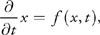
which says that the rate at which some quantity x is changing is given by some function f, which may itself depend on x and t. The reader may find it easier to think about this relationship in the discrete setting of forward Euler integration:
|
x n + 1 = xn + f(xn, tn )t. |
In other words, the value of x at the next time step equals the current value of x plus the current rate of change f (xn , tn ) times the duration of the time step t. (Note that superscripts are used to index the time step and do not imply exponentiation.) Be warned, however, that the forward Euler scheme is not a good choice numerically—we are suggesting it only as a way to think about the equations.
30.2.2 Equations of Fluid Motion
The motion of a fluid is often expressed in terms of its local velocity u as a function of position and time. In computer animation, fluid is commonly modeled as inviscid (that is, more like water than oil) and incompressible (meaning that volume does not change over time). Given these assumptions, the velocity can be described by the momentum equation:
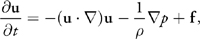
subject to the incompressibility constraint:
|
|
where p is the pressure, is the mass density, f represents any external
forces (such as gravity), and
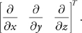
 is the differential operator:
To define the equations of motion in a particular context, it is also necessary to specify boundary conditions (that is, how the fluid behaves near solid obstacles or other fluids).
The basic task of a fluid solver is to compute a numerical approximation of u. This velocity field can then be used to animate visual phenomena such as smoke particles or a liquid surface.
30.2.3 Solving for Velocity
The popular "stable fluids" method for computing velocity was introduced in Stam 1999, and a GPU implementation of this method for 2D fluids was presented in Harris 2004. In this section we briefly describe how to solve for velocity but refer the reader to the cited works for details.
In order to numerically solve the momentum equation, we must discretize our domain (that is, the region of space through which the fluid flows) into computational elements. We choose an Eulerian discretization, meaning that computational elements are fixed in space throughout the simulation—only the values stored on these elements change. In particular, we subdivide a rectilinear volume into a regular grid of cubical cells. Each grid cell stores both scalar quantities (such as pressure, temperature, and so on) and vector quantities (such as velocity). This scheme makes implementation on the GPU simple, because there is a straightforward mapping between grid cells and voxels in a 3D texture. Lagrangian schemes (that is, schemes where the computational elements are not fixed in space) such as smoothed-particle hydrodynamics (Müller et al. 2003) are also popular for fluid animation, but their irregular structure makes them difficult to implement efficiently on the GPU.
Because we discretize space, we must also discretize derivatives in our equations: finite differences numerically approximate derivatives by taking linear combinations of values defined on the grid. As in Harris 2004, we store all quantities at cell centers for pedagogical simplicity, though a staggered MAC-style grid yields more-robust finite differences and can make it easier to define boundary conditions. (See Harlow and Welch 1965 for details.)
In a GPU implementation, cell attributes (velocity, pressure, and so on) are stored in several 3D textures. At each simulation step, we update these values by running computational kernels over the grid. A kernel is implemented as a pixel shader that executes on every cell in the grid and writes the results to an output texture. However, because GPUs are designed to render into 2D buffers, we must run kernels once for each slice of a 3D volume.
To execute a kernel on a particular grid slice, we rasterize a single quad whose dimensions equal the width and height of the volume. In Direct3D 10 we can directly render into a 3D texture by specifying one of its slices as a render target. Placing the slice index in a variable bound to the SV_RenderTargetArrayIndex semantic specifies the slice to which a primitive coming out of the geometry shader is rasterized. (See Blythe 2006 for details.) By iterating over slice indices, we can execute a kernel over the entire grid.
Rather than solve the momentum equation all at once, we split it into a set of simpler operations that can be computed in succession: advection, application of external forces, and pressure projection. Implementation of the corresponding kernels is detailed in Harris 2004, but several examples from our Direct3D 10 framework are given in Listing 30-1. Of particular interest is the routine PS_ADVECT_VEL: this kernel implements semi-Lagrangian advection, which is used as a building block for more accurate advection in the next section.
Example 30-1. Simulation Kernels
struct GS_OUTPUT_FLUIDSIM
{
  // Index of the current grid cell (i,j,k in [0,gridSize] range)
   float3 cellIndex : TEXCOORD0;
  // Texture coordinates (x,y,z in [0,1] range) for the
   // current grid cell and its immediate neighbors
   float3 CENTERCELL : TEXCOORD1;
  float3 LEFTCELL   : TEXCOORD2;
  float3 RIGHTCELL  : TEXCOORD3;
  float3 BOTTOMCELL : TEXCOORD4;
  float3 TOPCELL    : TEXCOORD5;
  float3 DOWNCELL   : TEXCOORD6;
  float3 UPCELL     : TEXCOORD7;
  float4 pos        : SV_Position; // 2D slice vertex in
   // homogeneous clip space
   uint RTIndex    : SV_RenderTargetArrayIndex;  // Specifies
   // destination slice
};
float3 cellIndex2TexCoord(float3 index)
{
  // Convert a value in the range [0,gridSize] to one in the range [0,1].
   return float3(index.x / textureWidth,
                index.y / textureHeight,
                (index.z+0.5) / textureDepth);
}
float4 PS_ADVECT_VEL(GS_OUTPUT_FLUIDSIM in,
                     Texture3D velocity) : SV_Target
{
  float3 pos = in.cellIndex;
  float3 cellVelocity = velocity.Sample(samPointClamp,
                                        in.CENTERCELL).xyz;
  pos -= timeStep * cellVelocity;
  pos = cellIndex2TexCoord(pos);
  return velocity.Sample(samLinear, pos);
}
float PS_DIVERGENCE(GS_OUTPUT_FLUIDSIM in,
                    Texture3D velocity) : SV_Target
{
  // Get velocity values from neighboring cells.
   float4 fieldL = velocity.Sample(samPointClamp, in.LEFTCELL);
  float4 fieldR = velocity.Sample(samPointClamp, in.RIGHTCELL);
  float4 fieldB = velocity.Sample(samPointClamp, in.BOTTOMCELL);
  float4 fieldT = velocity.Sample(samPointClamp, in.TOPCELL);
  float4 fieldD = velocity.Sample(samPointClamp, in.DOWNCELL);
  float4 fieldU = velocity.Sample(samPointClamp, in.UPCELL);
  // Compute the velocity's divergence using central differences.
   float divergence =  0.5 * ((fieldR.x - fieldL.x)+
                             (fieldT.y - fieldB.y)+
                             (fieldU.z - fieldD.z));
  return divergence;
}
float PS_JACOBI(GS_OUTPUT_FLUIDSIM in,
                Texture3D pressure,
                Texture3D divergence) : SV_Target
{
  // Get the divergence at the current cell.
   float dC = divergence.Sample(samPointClamp, in.CENTERCELL);
  // Get pressure values from neighboring cells.
   float pL = pressure.Sample(samPointClamp, in.LEFTCELL);
  float pR = pressure.Sample(samPointClamp, in.RIGHTCELL);
  float pB = pressure.Sample(samPointClamp, in.BOTTOMCELL);
  float pT = pressure.Sample(samPointClamp, in.TOPCELL);
  float pD = pressure.Sample(samPointClamp, in.DOWNCELL);
  float pU = pressure.Sample(samPointClamp, in.UPCELL);
  // Compute the new pressure value for the center cell.
   return(pL + pR + pB + pT + pU + pD - dC) / 6.0;
}
float4 PS_PROJECT(GS_OUTPUT_FLUIDSIM in,
                  Texture3D pressure,
                  Texture3D velocity): SV_Target
{
  // Compute the gradient of pressure at the current cell by
   // taking central differences of neighboring pressure values.
   float pL = pressure.Sample(samPointClamp, in.LEFTCELL);
  float pR = pressure.Sample(samPointClamp, in.RIGHTCELL);
  float pB = pressure.Sample(samPointClamp, in.BOTTOMCELL);
  float pT = pressure.Sample(samPointClamp, in.TOPCELL);
  float pD = pressure.Sample(samPointClamp, in.DOWNCELL);
  float pU = pressure.Sample(samPointClamp, in.UPCELL);
  float3 gradP = 0.5*float3(pR - pL, pT - pB, pU - pD);
  // Project the velocity onto its divergence-free component by
   // subtracting the gradient of pressure.
   float3 vOld = velocity.Sample(samPointClamp, in.texcoords);
  float3 vNew = vOld - gradP;
  return float4(vNew, 0);
}
Improving Detail
The semi-Lagrangian advection scheme used by Stam is useful for animation because it is unconditionally stable, meaning that large time steps will not cause the simulation to "blow up." However, it can introduce unwanted numerical smoothing, making water look viscous or causing smoke to lose detail. To achieve higher-order accuracy, we use a MacCormack scheme that performs two intermediate semi-Lagrangian advection steps. Given a quantity and an advection scheme A (for example, the one implemented by PS_ADVECT_VEL), higher-order accuracy is obtained using the following sequence of operations (from Selle et al. 2007):
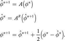
Here, n is the quantity to be advected,
) and
and
) are intermediate quantities, and n+1 is the final advected quantity. The superscript on
A R indicates that advection is reversed (that is, time is run backward) for that
step.
are intermediate quantities, and n+1 is the final advected quantity. The superscript on
A R indicates that advection is reversed (that is, time is run backward) for that
step.
Unlike the standard semi-Lagrangian scheme, this MacCormack scheme is not unconditionally stable. Therefore, a limiter is applied to the resulting value n+1, ensuring that it falls within the range of values contributing to the initial semi-Lagrangian advection. In our GPU solver, this means we must locate the eight nodes closest to the sample point, access the corresponding texels exactly at their centers (to avoid getting interpolated values), and clamp the final value to fall within the minimum and maximum values found on these nodes, as shown in Figure 30-2.
)
Figure 30-2 Limiter Applied to a MacCormack Advection Scheme in 2D
Once the intermediate semi-Lagrangian steps have been computed, the pixel shader in Listing 30-2 completes advection using the MacCormack scheme.
Example 30-2. MacCormack Advection Scheme
float4 PS_ADVECT_MACCORMACK(GS_OUTPUT_FLUIDSIM in,
                            float timestep) : SV_Target
{
  // Trace back along the initial characteristic - we'll use
   // values near this semi-Lagrangian "particle" to clamp our
   // final advected value.
   float3 cellVelocity = velocity.Sample(samPointClamp,
                                        in.CENTERCELL).xyz;
float3 npos = in.cellIndex - timestep * cellVelocity;
// Find the cell corner closest to the "particle" and compute the
   // texture coordinate corresponding to that location.
npos = floor(npos + float3(0.5f, 0.5f, 0.5f));
npos = cellIndex2TexCoord(npos);
// Get the values of nodes that contribute to the interpolated value.
   // Texel centers will be a half-texel away from the cell corner.
   float3 ht = float3(0.5f / textureWidth,
                   0.5f / textureHeight,
                   0.5f / textureDepth);
float4 nodeValues[8];
nodeValues[0] = phi_n.Sample(samPointClamp, npos +
                             float3(-ht.x, -ht.y, -ht.z));
nodeValues[1] = phi_n.Sample(samPointClamp, npos +
                             float3(-ht.x, -ht.y, ht.z));
nodeValues[2] = phi_n.Sample(samPointClamp, npos +
                             float3(-ht.x, ht.y, -ht.z));
nodeValues[3] = phi_n.Sample(samPointClamp, npos +
                             float3(-ht.x, ht.y, ht.z));
nodeValues[4] = phi_n.Sample(samPointClamp, npos +
                             float3(ht.x, -ht.y, -ht.z));
nodeValues[5] = phi_n.Sample(samPointClamp, npos +
                             float3(ht.x, -ht.y, ht.z));
nodeValues[6] = phi_n.Sample(samPointClamp, npos +
                             float3(ht.x, ht.y, -ht.z));
nodeValues[7] = phi_n.Sample(samPointClamp, npos +
                             float3(ht.x, ht.y, ht.z));
// Determine a valid range for the result.
   float4 phiMin = min(min(min(min(min(min(min(
    nodeValues[0],  nodeValues [1]), nodeValues [2]), nodeValues [3]),
    nodeValues[4]), nodeValues [5]), nodeValues [6]), nodeValues [7]);
float4 phiMax = max(max(max(max(max(max(max(
    nodeValues[0],  nodeValues [1]), nodeValues [2]), nodeValues [3]),
    nodeValues[4]), nodeValues [5]), nodeValues [6]), nodeValues [7]);
// Perform final advection, combining values from intermediate
   // advection steps.
   float4 r = phi_n_1_hat.Sample(samLinear, nposTC) +
           0.5 * (phi_n.Sample(samPointClamp, in.CENTERCELL) -
                  phi_n_hat.Sample(samPointClamp, in.CENTERCELL));
// Clamp result to the desired range.
r = max(min(r, phiMax), phiMin);
return r;
}
On the GPU, higher-order schemes are often a better way to get improved visual detail than simply increasing the grid resolution, because math is cheap compared to band-width. Figure 30-3 compares a higher-order scheme on a low-resolution grid with a lower-order scheme on a high-resolution grid.
)
Figure 30-3 Bigger Is Not Always Better!
30.2.4 Solid-Fluid Interaction
One of the benefits of using real-time simulation (versus precomputed animation) is that fluid can interact with the environment. Figure 30-4 shows an example on one such scene. In this section we discuss two simple ways to allow the environment to act on the fluid.
)
Figure 30-4 An Animated Gargoyle Pushes Smoke Around by Flapping Its Wings
A basic way to influence the velocity field is through the application of external forces. To get the gross
effect of an obstacle pushing fluid around, we can approximate the obstacle with a basic shape such as a box or
a ball and add the obstacle's average velocity to that region of the velocity field. Simple shapes like these
can be described with an implicit equation of the form f (x, y, z)
 0
that can be easily evaluated by a pixel shader at each grid cell.
0
that can be easily evaluated by a pixel shader at each grid cell.
Although we could explicitly add velocity to approximate simple motion, there are situations in which more detail is required. In Hellgate: London, for example, we wanted smoke to seep out through cracks in the ground. Adding a simple upward velocity and smoke density in the shape of a crack resulted in uninteresting motion. Instead, we used the crack shape, shown inset in Figure 30-5, to define solid obstacles for smoke to collide and interact with. Similarly, we wanted to achieve more-precise interactions between smoke and an animated gargoyle, as shown in Figure 30-4. To do so, we needed to be able to affect the fluid motion with dynamic obstacles (see the details later in this section), which required a volumetric representation of the obstacle's interior and of the velocity at its boundary (which we also explain later in this section).
)
Figure 30-5 Smoke Rises from a Crack in the Ground in the Game
Dynamic Obstacles
So far we have assumed that a fluid occupies the entire rectilinear region defined by the simulation grid. However, in most applications, the fluid domain (that is, the region of the grid actually occupied by fluid) is much more interesting. Various methods for handling static boundaries on the GPU are discussed in Harris et al. 2003, Liu et al. 2004, Wu et al. 2004, and Li et al. 2005.
The fluid domain may change over time to adapt to dynamic obstacles in the environment, and in the case of liquids, such as water, the domain is constantly changing as the liquid sloshes around (more in Section 30.2.7). In this section we describe the scheme used for handling dynamic obstacles in Hellgate: London. For further discussion of dynamic obstacles, see Bridson et al. 2006 and Foster and Fedkiw 2001.
To deal with complex domains, we must consider the fluid's behavior at the domain boundary. In our discretized fluid, the domain boundary consists of the faces between cells that contain fluid and cells that do not—that is, the face between a fluid cell and a solid cell is part of the boundary, but the solid cell itself is not. A simple example of a domain boundary is a static barrier placed around the perimeter of the simulation grid to prevent fluid from "escaping" (without it, the fluid appears as though it is simply flowing out into space).
To support domain boundaries that change due to the presence of dynamic obstacles, we need to modify some of our simulation steps. In our implementation, obstacles are represented using an inside-outside voxelization. In addition, we keep a voxelized representation of the obstacle's velocity in solid cells adjacent to the domain boundary. This information is stored in a pair of 3D textures that are updated whenever an obstacle moves or deforms (we cover this later in this section).
At solid-fluid boundaries, we want to impose a free-slip boundary condition, which says that the velocities of the fluid and the solid are the same in the direction normal to the boundary:
|
u · n = u solid · n. |
In other words, the fluid cannot flow into or out of a solid, but it is allowed to flow freely along its surface.
The free-slip boundary condition also affects the way we solve for pressure, because the gradient of pressure is used in determining the final velocity. A detailed discussion of pressure projection can be found in Bridson et al. 2006, but ultimately we just need to make sure that the pressure values we compute satisfy the following:
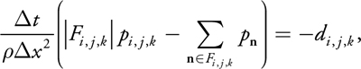
where t is the size of the time step, x is the cell spacing, pi
, j , k is the pressure value in cell (i,
j, k), di , j ,
k is the discrete velocity divergence computed for that cell, and Fi
, j , k is the set of indices of cells
adjacent to cell (i, j, k) that contain fluid. (This equation is simply a discrete
form of the pressure-Poisson system
2
p
=
· w in Harris 2004 that respects solid boundaries.) It is also important that at solid-fluid
boundaries, di , j , k is
computed using obstacle velocities.
In practice there's a very simple trick for making sure all this happens: any time we sample pressure from a neighboring cell (for example, in the pressure solve and pressure projection steps), we check whether the neighbor contains a solid obstacle, as shown in Figure 30-6. If it does, we use the pressure value from the center cell in place of the neighbor's pressure value. In other words, we nullify the solid cell's contribution to the preceding equation.
)
Figure 30-6 Accounting for Obstacles in the Computation of the Discrete Laplacian of Pressure
We can apply a similar trick for velocity values: whenever we sample a neighboring cell (for example, when computing the velocity's divergence), we first check to see if it contains a solid. If so, we look up the obstacle's velocity from our voxelization and use it in place of the value stored in the fluid's velocity field.
Because we cannot always solve the pressure-Poisson system to convergence, we explicitly enforce the free-slip boundary condition immediately following pressure projection. We must also correct the result of the pressure projection step for fluid cells next to the domain boundary. To do so, we compute the obstacle's velocity component in the direction normal to the boundary. This value replaces the corresponding component of our fluid velocity at the center cell, as shown in Figure 30-7. Because solid-fluid boundaries are aligned with voxel faces, computing the projection of the velocity onto the surface normal is simply a matter of selecting the appropriate component.
)
Figure 30-7 Enforcing the Free-Slip Boundary Condition After Pressure Projection
If two opposing faces of a fluid cell are solid-fluid boundaries, we could average the velocity values from both sides. However, simply selecting one of the two faces generally gives acceptable results.
Finally, it is important to realize that when very large time steps are used, quantities can "leak" through boundaries during advection. For this reason we add an additional constraint to the advection steps to ensure that we never advect any quantity into the interior of an obstacle, guaranteeing that the value of advected quantities (for example, smoke density) is always zero inside solid obstacles (see the PS_ADVECT_OBSTACLE routine in Listing 30-3). In Listing 30-3, we show the simulation kernels modified to take boundary conditions into account.
Example 30-3. Modified Simulation Kernels to Account for Boundary Conditions
bool IsSolidCell(float3 cellTexCoords)
{
  return obstacles.Sample(samPointClamp, cellTexCoords).r > 0.9;
}
float PS_JACOBI_OBSTACLE(GS_OUTPUT_FLUIDSIM in,
                         Texture3D pressure,
                         Texture3D divergence) : SV_Target
{
  // Get the divergence and pressure at the current cell.
   float dC = divergence.Sample(samPointClamp, in.CENTERCELL);
  float pC = pressure.Sample(samPointClamp, in.CENTERCELL);
  // Get the pressure values from neighboring cells.
   float pL = pressure.Sample(samPointClamp, in.LEFTCELL);
  float pR = pressure.Sample(samPointClamp, in.RIGHTCELL);
  float pB = pressure.Sample(samPointClamp, in.BOTTOMCELL);
  float pT = pressure.Sample(samPointClamp, in.TOPCELL);
  float pD = pressure.Sample(samPointClamp, in.DOWNCELL);
  float pU = pressure.Sample(samPointClamp, in.UPCELL);
  // Make sure that the pressure in solid cells is effectively ignored.
   if(IsSolidCell(in.LEFTCELL)) pL = pC;
  if(IsSolidCell(in.RIGHTCELL)) pR = pC;
  if(IsSolidCell(in.BOTTOMCELL)) pB = pC;
  if(IsSolidCell(in.TOPCELL)) pT = pC;
  if(IsSolidCell(in.DOWNCELL)) pD = pC;
  if(IsSolidCell(in.UPCELL)) pU = pC;
  // Compute the new pressure value.
   return(pL + pR + pB + pT + pU + pD - dC) /6.0;
}
float4 GetObstacleVelocity(float3 cellTexCoords)
{
  return obstaclevelocity.Sample(samPointClamp, cellTexCoords);
}
float PS_DIVERGENCE_OBSTACLE(GS_OUTPUT_FLUIDSIM in,
                             Texture3D velocity) : SV_Target
{
  // Get velocity values from neighboring cells.
   float4 fieldL = velocity.Sample(samPointClamp, in.LEFTCELL);
  float4 fieldR = velocity.Sample(samPointClamp, in.RIGHTCELL);
  float4 fieldB = velocity.Sample(samPointClamp, in.BOTTOMCELL);
  float4 fieldT = velocity.Sample(samPointClamp, in.TOPCELL);
  float4 fieldD = velocity.Sample(samPointClamp, in.DOWNCELL);
  float4 fieldU = velocity.Sample(samPointClamp, in.UPCELL);
  // Use obstacle velocities for any solid cells.
   if(IsBoundaryCell(in.LEFTCELL))
    fieldL = GetObstacleVelocity(in.LEFTCELL);
  if(IsBoundaryCell(in.RIGHTCELL))
    fieldR = GetObstacleVelocity(in.RIGHTCELL);
  if(IsBoundaryCell(in.BOTTOMCELL))
   fieldB = GetObstacleVelocity(in.BOTTOMCELL);
  if(IsBoundaryCell(in.TOPCELL))
   fieldT = GetObstacleVelocity(in.TOPCELL);
  if(IsBoundaryCell(in.DOWNCELL))
   fieldD = GetObstacleVelocity(in.DOWNCELL);
  if(IsBoundaryCell(in.UPCELL))
   fieldU = GetObstacleVelocity(in.UPCELL);
  // Compute the velocity's divergence using central differences.
   float divergence =  0.5 * ((fieldR.x - fieldL.x) +
                             (fieldT.y - fieldB.y) +
                             (fieldU.z - fieldD.z));
  return divergence;
}
float4 PS_PROJECT_OBSTACLE(GS_OUTPUT_FLUIDSIM in,
                           Texture3D pressure,
                           Texture3D velocity): SV_Target
{
  // If the cell is solid, simply use the corresponding
   // obstacle velocity.
   if(IsBoundaryCell(in.CENTERCELL))
  {
    return GetObstacleVelocity(in.CENTERCELL);
  }
  // Get pressure values for the current cell and its neighbors.
   float pC = pressure.Sample(samPointClamp, in.CENTERCELL);
  float pL = pressure.Sample(samPointClamp, in.LEFTCELL);
  float pR = pressure.Sample(samPointClamp, in.RIGHTCELL);
  float pB = pressure.Sample(samPointClamp, in.BOTTOMCELL);
  float pT = pressure.Sample(samPointClamp, in.TOPCELL);
  float pD = pressure.Sample(samPointClamp, in.DOWNCELL);
  float pU = pressure.Sample(samPointClamp, in.UPCELL);
  // Get obstacle velocities in neighboring solid cells.
   // (Note that these values are meaningless if a neighbor
   // is not solid.)
   float3 vL = GetObstacleVelocity(in.LEFTCELL);
  float3 vR = GetObstacleVelocity(in.RIGHTCELL);
  float3 vB = GetObstacleVelocity(in.BOTTOMCELL);
  float3 vT = GetObstacleVelocity(in.TOPCELL);
  float3 vD = GetObstacleVelocity(in.DOWNCELL);
  float3 vU = GetObstacleVelocity(in.UPCELL);
  float3 obstV = float3(0,0,0);
  float3 vMask = float3(1,1,1);
  // If an adjacent cell is solid, ignore its pressure
   // and use its velocity.
   if(IsBoundaryCell(in.LEFTCELL)) {
    pL = pC; obstV.x = vL.x; vMask.x = 0; }
  if(IsBoundaryCell(in.RIGHTCELL)) {
    pR = pC; obstV.x = vR.x; vMask.x = 0; }
  if(IsBoundaryCell(in.BOTTOMCELL)) {
    pB = pC; obstV.y = vB.y; vMask.y = 0; }
  if(IsBoundaryCell(in.TOPCELL)) {
    pT = pC; obstV.y = vT.y; vMask.y = 0; }
  if(IsBoundaryCell(in.DOWNCELL)) {
    pD = pC; obstV.z = vD.z; vMask.z = 0; }
  if(IsBoundaryCell(in.UPCELL)) {
    pU = pC; obstV.z = vU.z; vMask.z = 0; }
  // Compute the gradient of pressure at the current cell by
   // taking central differences of neighboring pressure values.
   float gradP = 0.5*float3(pR - pL, pT - pB, pU - pD);
  // Project the velocity onto its divergence-free component by
   // subtracting the gradient of pressure.
   float3 vOld = velocity.Sample(samPointClamp, in.texcoords);
  float3 vNew = vOld - gradP;
  // Explicitly enforce the free-slip boundary condition by
   // replacing the appropriate components of the new velocity with
   // obstacle velocities.
  vNew = (vMask * vNew) + obstV;
  return vNew;
}
bool IsNonEmptyCell(float3 cellTexCoords)
{
  return obstacles.Sample(samPointClamp, cellTexCoords, 0).r > 0.0);
}
float4 PS_ADVECT_OBSTACLE(GS_OUTPUT_FLUIDSIM in,
                          Texture3D velocity,
                          Texture3D color) : SV_Target
{
  if(IsNonEmptyCell(in.CENTERCELL))
  {
    return 0;
  }
  float3 cellVelocity = velocity.Sample(samPointClamp,
                                        in.CENTERCELL).xyz;
  float3 pos = in.cellIndex - timeStep*cellVelocity;
  float3 npos = float3(pos.x / textureWidth,
                       pos.y / textureHeight,
                       (pos.z+0.5) / textureDepth);
  return color.Sample(samLinear, npos);
}
Voxelization
To handle boundary conditions for dynamic solids, we need a quick way of determining whether a given cell contains a solid obstacle. We also need to know the solid's velocity for cells next to obstacle boundaries. To do this, we voxelize solid obstacles into an "inside-outside" texture and an "obstacle velocity" texture, as shown in Figure 30-8, using two different voxelization routines.
)
Figure 30-8 Solid Obstacles Are Voxelized into an Inside-Outside Texture and an Obstacle Velocity Texture
Inside-Outside Voxelization
Our approach to obtain an inside-outside voxelization is inspired by the stencil shadow volumes algorithm. The idea is simple: We render the input triangle mesh once into each slice of the destination 3D texture using an orthogonal projection. The far clip plane is set at infinity, and the near plane matches the depth of the current slice, as shown in Figure 30-9. When drawing geometry, we use a stencil buffer (of the same dimensions as the slice) that is initialized to zero. We set the stencil operations to increment for back faces and decrement for front faces (with wrapping in both cases). The result is that any voxel inside the mesh receives a nonzero stencil value. We then do a final pass that copies stencil values into the obstacle texture. [1]
)
Figure 30-9 Inside-Outside Voxelization of a Mesh
As a result, we are able to distinguish among three types of cells: interior (nonzero stencil value), exterior (zero stencil), and interior but next to the boundary (these cells are tagged by the velocity voxelization algorithm, described next). Note that because this method depends on having one back face for every front face, it is best suited to water-tight closed meshes.
Velocity Voxelization
The second voxelization algorithm computes an obstacle's velocity at each grid cell that contains part of the obstacle's boundary. First, however, we need to know the obstacle's velocity at each vertex. A simple way to compute per-vertex velocities is to store vertex positions p n-1 and p n from the previous and current frames, respectively, in a vertex buffer. The instantaneous velocity v i of vertex i can be approximated with the forward difference
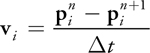
in a vertex shader.
Next, we must compute interpolated obstacle velocities for any grid cell containing a piece of a surface mesh. As with the inside-outside voxelization, the mesh is rendered once for each slice of the grid. This time, however, we must determine the intersection of each triangle with the current slice.
The intersection between a slice and a triangle is a segment, a triangle, a point, or empty. If the intersection is a segment, we draw a "thickened" version of the segment into the slice using a quad. This quad consists of the two end points of the original segment and two additional points offset from these end points, as shown in Figure 30-10. The offset distance w is equal to the diagonal length of one texel in a slice of the 3D texture, and the offset direction is the projection of the triangle's normal onto the slice. Using linear interpolation, we determine velocity values at each end point and assign them to the corresponding vertices of the quad. When the quad is drawn, these values get interpolated across the grid cells as desired.
)
Figure 30-10 A Triangle Intersects a Slice at a Segment with End Points and .
These quads can be generated using a geometry shader that operates on mesh triangles, producing four vertices if the intersection is a segment and zero vertices otherwise. Because geometry shaders cannot output quads, we must instead use a two-triangle strip. To compute the triangle-slice intersection, we intersect each triangle edge with the slice. If exactly two edge-slice intersections are found, the corresponding intersection points are used as end points for our segment. Velocity values at these points are computed via interpolation along the appropriate triangle edges. The geometry shader GS_GEN_BOUNDARY_VELOCITY in Listing 30-4 gives an implementation of this algorithm. Figure 30-12 shows a few slices of a voxel volume resulting from the voxelization of the model in Figure 30-11.
)
Figure 30-11 Simplified Geometry Can Be Used to Speed Up Voxelization
)
Figure 30-12 Slices of the 3D Textures Resulting from Applying Our Voxelization Algorithms to the Model in .
Example 30-4. Geometry Shader for Velocity Voxelization
   // GS_GEN_BOUNDARY_VELOCITY:
   // Takes as input:
   //  - one triangle (3 vertices),
   //  - the sliceIdx,
   //  - the sliceZ;
   // and outputs:
   //  - 2 triangles, if intersection of input triangle with slice
   //    is a segment
   //  - 0 triangles, otherwise
   // The 2 triangles form a 1-voxel wide quadrilateral along the
   // segment.
[maxvertexcount (4)]
void GS_GEN_BOUNDARY_VELOCITY(
  triangle VsGenVelOutput input[3],
  inout TriangleStream<GsGenVelOutput> triStream)
{
  GsGenVelOutput output;
  output.RTIndex = sliceIdx;
  float minZ = min(min(input[0].Pos.z, input[1].Pos.z), input[2].Pos.z);
  float maxZ = max(max(input[0].Pos.z, input[1].Pos.z), input[2].Pos.z);
  if((sliceZ < minZ) || (sliceZ > maxZ))
    // This triangle doesn't intersect the slice.
   return;
  GsGenVelIntVtx intersections[2];
  for(int i=0; i<2; i++)
  {
    intersections[i].Pos = 0;
    intersections[i].Velocity = 0;
  }
  int idx = 0;
  if(idx < 2)
    GetEdgePlaneIntersection(input[0], input[1], sliceZ,
                             intersections, idx);
  if(idx < 2)
    GetEdgePlaneIntersection(input[1], input[2], sliceZ,
                             intersections, idx);
  if(idx < 2)
    GetEdgePlaneIntersection(input[2], input[0], sliceZ,
                             intersections, idx);
  if(idx < 2)
    return;
  float sqrtOf2 = 1.414; // The diagonal of a pixel
   float2 normal = sqrtOf2 * normalize(
    cross((input[1].Pos - input[0].Pos),
          (input[2].Pos - input[0].Pos)).xy);
  for(int i=0; i<2; i++)
  {
    output.Pos = float4(intersections[i].Pos, 0, 1);
    output.Velocity = intersections[i].Velocity;
    triStream.Append(output);
    output.Pos = float4((intersections[i].Pos +
                        (normal*projSpacePixDim)), 0, 1);
    output.Velocity = intersections[i].Velocity;
    triStream.Append(output);
  }
  triStream.RestartStrip();
}
void GetEdgePlaneIntersection(
  VsGenVelOutput vA,
  VsGenVelOutput vB,
  float sliceZ,
  inout GsGenVelIntVtx intersections[2],
  inout int idx)
{
  float t = (sliceZ - vA.Pos.z) / (vB.Pos.z - vA.Pos.z);
  if((t < 0) || (t > 1))
    // Line-plane intersection is not within the edge's end points
   // (A and B)
   return;
    intersections[idx].Pos = lerp(vA.Pos, vB.Pos, t).xy;
    intersections[idx].Velocity = lerp(vA.Velocity, vB.Velocity, t);
    idx++;
}
Optimizing Voxelization
Although voxelization requires a large number of draw calls, it can be made more efficient using stream output(see Blythe 2006). Stream output allows an entire buffer of transformed vertices to be cached when voxelizing deforming meshes such as skinned characters, rather than recomputing these transformations for each slice.
Additionally, instancing can be used to draw all slices in a single draw call, rather than making a separate call for each slice. In this case, the instance ID can be used to specify the target slice.
Due to the relative coarseness of the simulation grid used, it is a good idea to use a low level of detail mesh for each obstacle, as shown in Figure 30-11. Using simplified models allowed us to voxelize obstacles at every frame with little performance cost.
Finally, if an obstacle is transformed by a simple analytic transformation (versus a complex skinning operation, for example), voxelization can be precomputed and the inverse of the transformation can be applied whenever accessing the 3D textures. A simple example is a mesh undergoing rigid translation and rotation: texture coordinates used to access the inside-outside and obstacle velocity textures can be multiplied by the inverse of the corresponding transformation matrix to get the appropriate values.
30.2.5 Smoke
Although the velocity field describes the fluid's motion, it does not look much like a fluid when visualized directly. To get interesting visual effects, we must keep track of additional quantities that are pushed around by the fluid. For instance, we can keep track of density and temperature to obtain the appearance of smoke (Fedkiw et al. 2001). For each additional quantity , we must allocate an additional texture with the same dimensions as our grid. The evolution of values in this texture is governed by the same advection equation used for velocity:
In other words, we can use the same MacCormack advection routine we used to evolve the velocity.
To achieve the particular effect seen in Figure 30-4, for example, we inject a three-dimensional Gaussian "splat" into a color texture each frame to provide a source of "smoke." These color values have no real physical significance, but they create attractive swirling patterns as they are advected throughout the volume by the fluid velocity.
To get a more physically plausible appearance, we must make sure that hot smoke rises and cool smoke falls. To do so, we need to keep track of the fluid temperature T (which again is advected by u). Unlike color, temperature values have an influence on the dynamics of the fluid. This influence is described by the buoyant force:
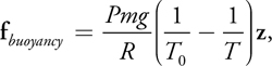
where P is pressure, m is the molar mass of the gas, g is the acceleration due to gravity, and R is the universal gas constant. In practice, all of these physical constants can be treated as a single value and can be tweaked to achieve the desired visual appearance. The value T 0 is the ambient or "room" temperature, and T represents the temperature values being advected through the flow. z is the normalized upward-direction vector. The buoyant force should be thought of as an "external" force and should be added to the velocity field immediately following velocity advection.
30.2.6 Fire
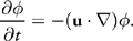
Fire is not very different from smoke except that we must store an additional quantity, called the reaction coordinate, that keeps track of the time elapsed since gas was ignited. A reaction coordinate of one indicates that the gas was just ignited, and a coordinate of less than zero indicates that the fuel has been completely exhausted. The evolution of these values is described by the following equation (from Nguyen et al. 2002):
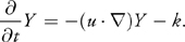
In other words, the reaction coordinate is advected through the flow and decremented by a constant amount (k) at each time step. In practice, this integration is performed by passing a value for k to the advection routine (PS_ADVECT_MACCORMACK), which is added to the result of the advection. (This value should be nonzero only when advecting the reaction coordinate.) Reaction coordinates do not have an effect on the dynamics of the fluid but are later used for rendering (see Section 30.3).
Figure 30-14 (in Section 30.2.10) demonstrates one possible fire effect: a ball of fuel is continuously generated near the bottom of the volume by setting the reaction coordinate in a spherical region to one. For a more advanced treatment of flames, see Nguyen et al. 2002.
30.2.7 Water
Water is modeled differently from the fluid phenomena discussed thus far. With fire or smoke, we are interested in visualizing a density defined throughout the entire volume, but with water the visually interesting part is the interface between air and liquid.
Therefore, we need some way of representing this interface and tracking how it deforms as it is pushed around by the fluid velocity.
The level set method (Sethian 1999) is a popular representation of a liquid surface and is particularly well suited to a GPU implementation because it requires only a scalar value at each grid cell. In a level set, each cell records the shortest signed distance from the cell center to the water surface. Cells in the grid are classified according to the value of : if < 0, the cell contains water; otherwise, it contains air. Wherever equals zero is exactly where the water meets the air (the zero set). Because advection will not preserve the distance field property of a level set, it is common to periodically reinitialize the level set. Reinitialization ensures that each cell does indeed store the shortest distance to the zero set. However, this property isn't needed to simply define the surface, and for real-time animation, it is possible to get decent results without reinitialization. Figure 30-1, at the beginning of this chapter, shows the quality of the results.
Just as with color, temperature, and other attributes, the level set is advected by the fluid, but it also
affects the simulation dynamics. In fact, the level set defines the fluid domain: in simple models of
water and air, we assume that the air has a negligible effect on the liquid and do not perform simulation
wherever
 0. In practice, this means we set the pressure outside of the liquid to zero before solving for pressure and
modify the pressure only in liquid cells. It also means that we do not apply external forces such as gravity
outside of the liquid. To make sure that only fluid cells are processed, we check the value of the level set
texture in the relevant shaders and mask computations at a cell if the value of f is above some
threshold. Two alternatives that may be more efficient are to use z-cull to eliminate cells (if the GPU does not
support dynamic flow control) (Sander et al. 2004) and to use a sparse data structure (Lefohn et al. 2004).
0. In practice, this means we set the pressure outside of the liquid to zero before solving for pressure and
modify the pressure only in liquid cells. It also means that we do not apply external forces such as gravity
outside of the liquid. To make sure that only fluid cells are processed, we check the value of the level set
texture in the relevant shaders and mask computations at a cell if the value of f is above some
threshold. Two alternatives that may be more efficient are to use z-cull to eliminate cells (if the GPU does not
support dynamic flow control) (Sander et al. 2004) and to use a sparse data structure (Lefohn et al. 2004).
30.2.8 Performance Considerations
One major factor in writing an efficient solver is bandwidth. For each frame of animation, the solver runs a large number of arithmetically simple kernels, in between which data must be transferred to and from texture memory. Although most of these kernels exhibit good locality, bandwidth is still a major issue: using 32-bit floating-point textures to store quantities yields roughly half the performance of 16-bit textures. Surprisingly, there is little visually discernible degradation that results from using 16-bit storage, as is shown in Figure 30-13. Note that arithmetic operations are still performed in 32-bit floating point, meaning that results are periodically truncated as they are written to the destination textures.
)
Figure 30-13 Smoke Simulated Using 16-Bit () and 32-Bit () Floating-Point Textures for Storage
In some cases it is tempting to store multiple cell attributes in a single texture in order to reduce memory usage or for convenience, but doing so is not always optimal in terms of memory bandwidth. For instance, suppose we packed both inside-outside and velocity information about an obstacle into a single RGBA texture. Iteratively solving the pressure-Poisson equation requires that we load inside-outside values numerous times each frame, but meanwhile the obstacle's velocity would go unused. Because packing these two textures together requires four times as many bytes transferred from memory as well as cache space, it may be wise to keep the obstacle's inside-outside information in its own scalar texture.
30.2.9 Storage
Table 30-1 gives some of the storage requirements needed for simulating and rendering fluids, which amounts to 41 bytes per cell for simulation and 20 bytes per pixel for rendering. However, most of this storage is required only temporarily while simulating or rendering, and hence it can be shared among multiple fluid simulations. In Hellgate: London, we stored the exclusive textures (the third column of the table) with each instance of smoke, but we created global versions of the rest of the textures (the last column of the table), which were shared by all the smoke simulations.
Table 30-1. Storage Needed for Simulating and Rendering Fluids
|
Total Space |
Exclusive Textures |
Shared Textures |
|
|
Fluid Simulation |
32 bytes per cell |
12 bytes per cell 1xRGBA16 (velocity) 2xR16 (pressure and density) |
20 bytes per cell 2xRGBA16 (temporary) 2xR16 (temporary) |
|
Voxelization |
9 bytes per cell |
— |
9 bytes per cell 1xRGBA16 (velocity) 1xR8 (inside-outside) |
|
Rendering |
20 bytes per pixel |
— |
20 bytes per pixel of off-screen render target 1xRGBA32 (ray data) 1xR32 (scene depth) |
30.2.10 Numerical Issues
Because real-time applications are so demanding, we have chosen the simplest numerical schemes that still give acceptable visual results. Note, however, that for high-quality animation, more accurate alternatives are preferable.
One of the most expensive parts of the simulation is solving the pressure-Poisson system,
2
p =
·
u*. We use the Jacobi method to solve this system because it is easy to implement efficiently
on the GPU. However, several other suitable solvers have been implemented on the GPU, including the Conjugate
Gradient method (Bolz et al. 2003) and the Multigrid method (Goodnight et al. 2003). Cyclic reduction is a
particularly interesting option because it is direct and can take advantage of banded systems (Kass et al.
2006). When picking an iterative solver, it may be worth considering not only the overall rate of convergence
but also the convergence rate of different spatial frequencies in the residual (Briggs et al. 2000).
Because there may not be enough time to reach convergence in a real-time application, the distribution of
frequencies will have some impact on the appearance of the solution.
Ideally we would like to solve the pressure-Poisson system exactly in order to satisfy the incompressibility constraint and preserve fluid volume. For fluids like smoke and fire, however, a change in volume does not always produce objectionable visual artifacts. Hence we can adjust the number of iterations when solving this system according to available resources. Figure 30-14 compares the appearance of a flame using different numbers of Jacobi iterations. Seen in motion, spinning vortices tend to "flatten out" a bit more when using only a small number of iterations, but the overall appearance is very similar.
)
Figure 30-14 Fire Simulation Using 20 Jacobi Iterations () and 1,000 Jacobi Iterations () for the Pressure Solve
For a more thorough discussion of GPGPU performance issues, see Pharr 2005.
For liquids, on the other hand, a change of volume is immediately apparent: fluid appears to either pour out from nowhere or disappear entirely! Even something as simple as water sitting in a tank can potentially be problematic if too few iterations are used to solve for pressure: because information does not travel from the tank floor to the water surface, pressure from the floor cannot counteract the force of gravity. As a result, the water slowly sinks through the bottom of the tank, as shown in Figure 30-15.
)
Figure 30-15 Uncorrected Water Simulation
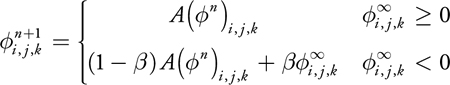
Unfortunately, in a real-time application, it is not always possible to solve for p exactly (regardless of the particular solver used) because computation time is constrained by the target frame rate and the resource requirements of other concurrent processes. In simple situations where we know that the liquid should tend toward a static equilibrium, we can force the correct behavior by manipulating the level set in the following way:
Here
 is a level set whose zero set tells us what the surface should look like if we let the liquid settle
for a long period of time. For example, the equilibrium level set for a tank of water would be simply f
(x, y, z) = y - h, where y is the vertical distance from
the bottom of the tank and h is the desired height of the water. See
Figure 30-16.
is a level set whose zero set tells us what the surface should look like if we let the liquid settle
for a long period of time. For example, the equilibrium level set for a tank of water would be simply f
(x, y, z) = y - h, where y is the vertical distance from
the bottom of the tank and h is the desired height of the water. See
Figure 30-16.
)
Figure 30-16 Combining Level Sets to Counter a Low Convergence Rate
The function A is the advection operator, and the parameter
 [0, 1] controls the amount of damping applied to the solution we get from advection. Larger values of
b permit fewer solver iterations but also decrease the liveliness of the fluid. Note that this damping
is applied only in regions of the domain where
is negative—this keeps splashes evolving outside of the domain of the equilibrium solution lively,
though it can result in temporary volume gain.
[0, 1] controls the amount of damping applied to the solution we get from advection. Larger values of
b permit fewer solver iterations but also decrease the liveliness of the fluid. Note that this damping
is applied only in regions of the domain where
is negative—this keeps splashes evolving outside of the domain of the equilibrium solution lively,
though it can result in temporary volume gain.
Ultimately, however, this kind of nonphysical manipulation of the level set is a hack, and its use should be considered judiciously. Consider an environment in which the player scoops up water with a bowl and then sets the bowl down at an arbitrary location on a table: we do not know beforehand what the equilibrium level set should look like and hence cannot prevent water from sinking through the bottom of the bowl.
30.3 Rendering
30.3.1 Volume Rendering
The result of our simulation is a collection of values stored in a 3D texture. However, there is no mechanism in Direct3D or OpenGL for displaying this texture directly. Therefore we render the fluid using a ray-marching pixel shader. Our approach is very similar to the one described in Scharsach 2005.
The placement of the fluid in the scene is determined by six quads, which represent the faces of the simulation volume. These quads are drawn into a deferred shading buffer to determine where and how rays should be cast. We then render the fluid by marching rays through the volume and accumulating densities from the 3D texture, as shown in Figure 30-17.
)
Figure 30-17 A Conceptual Overview of Ray Casting
Volume Ray Casting
In order to cast a ray, we need to know where it enters the volume, in which direction it is traveling, and how many samples to take. One way to get these values is to perform several ray-plane intersections in the ray-marching shader. However, precomputing these values and storing them in a texture makes it easier to perform proper compositing and clipping (more on this later in this section), which is the approach we use here. As a prepass, we generate a screen-size texture, called the RayData texture, which encodes, for every pixel that is to be rendered, the entry point of the ray in texture space, and the depth through the volume that the ray traverses. To get the depth through the volume, we draw first the back faces of the volume with a shader that outputs the distance from the eye to the fragment's position (in view space) into the alpha channel. We then run a similar shader on the front faces but enable subtractive blending using Equation 1. Furthermore, to get the entry point of the ray, we also output into the RGB channel the texture-space coordinates of each fragment generated for the front faces.
Equation 1

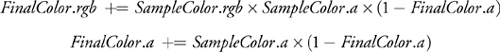
To render the volume, we draw a full-screen quad with a ray-marching shader. This shader looks up into the RayData texture to find the pixels that we need to ray-cast through, and the ray entry point and marching distance through the volume for those pixels. The number of samples that the ray-marching shader uses is proportional to the marching distance (we use a step size equal to half a voxel). The ray direction is given by the vector from the eye to the entry point (both in texture space). At each step along the ray, we sample values from the texture containing the simulated values and blend them front to back according to Equation 2. By blending from front to back, we can terminate ray casting early if the color saturates (we exit if FinalColor.a > 0.99). For a more physically based rendering model, see Fedkiw et al. 2001.
Equation 2
Compositing
There are two problems with the ray-marching algorithm described so far. First, rays continue to march through the volume even if they encounter other scene geometry. See the right side of Figure 30-18 for an illustration. Second, rays are traced even for parts of the volume that are completely occluded, as the left side of Figure 30-18 shows. However, we can modify our computation of volume depth such that we march through only relevant parts of the grid.
)
Figure 30-18 Rays Are Clipped According to Scene Depth to Account for Occlusion
Previously we used the distance to the back faces of the volume to determine where ray marching should terminate. To handle obstacles that intersect the volume, we instead use the minimum of the back-face distance and the scene distance (that is, the distance between the eye and the closest obstacle in the scene). The scene distance can be calculated by reading the scene depth and reverse projecting it back to view space to find the distance from the eye to the scene. If the depth buffer cannot be read as a texture in a pixel shader, as is the case in Direct3D 10 when using multisample antialiasing, this distance can be computed in the main scene rendering pass using multiple render targets; this is the approach we use.
To deal with cases in which the scene geometry completely occludes part of the volume, we compare the front-facing fragments' distance to the scene distance. If the front-face distance is greater than the scene distance (that is, the fragment is occluded), we output a large negative value in the red channel. This way, the final texture-space position computed for the corresponding texel in the RayData texture will be outside the volume, and hence no samples will be taken along the corresponding ray.
Clipping
We also need to modify our ray-marching algorithm to handle the cases in which the camera is located inside the fluid volume and the camera's near plane clips parts of the front faces of the volume, as shown in Figure 30-19.
)
Figure 30-19 Part of the Fluid Volume May Be Clipped by the Near Plane
In regions where the front faces were clipped, we have no information about where rays enter the volume, and we have incorrect values for the volume depth.
To deal with these regions, we mark the pixels where the back faces of the volume have been rendered but not the front faces. This marking is done by writing a negative color value into the green channel when rendering the back faces of the fluid volume to the RayData texture. Note that the RayData texture is cleared to zero before either front or back faces are rendered to it. Because we do not use the RGB values of the destination color when rendering the front faces with alpha blending (Equation 1), the pixels for which the green channel contains a negative color after rendering the front faces are those where the back faces of the fluid volume were rendered but not the front (due to clipping). In the ray-casting shader, we explicitly initialize the position of these marked pixels to the appropriate texture-space position of the corresponding point on the near plane. We also correct the depth value read from the RayData texture by subtracting from it the distance from the eye to the corresponding point on the near plane.
Filtering
The ray-marching algorithm presented so far has several visible artifacts. One such artifact is banding, which results from using an integral number of equally spaced samples. This artifact is especially visible when the scene inside the fluid volume has rapidly changing depth values, as illustrated in Figure 30-20.
)
Figure 30-20 Dealing with Banding
To suppress it, we take one more sample than necessary and weigh its contribution to the final color by d/sampleWidth, as shown in Figure 30-21. In the figure, d is the difference between the scene distance at the fragment and the total distance traveled by the ray at the last sample, and sampleWidth is the typical step size along the ray.
)
Figure 30-21 Reducing Banding by Taking an Additional Weighted Sample
Banding, however, usually remains present to some degree and can become even more obvious with high-frequency variations in either the volume density or the mapping between density and color (known as the transfer function). This well-known problem is addressed in Hadwiger 2004 and Sigg and Hadwiger 2005. Common solutions include increasing the sampling frequency, jittering the samples along the ray direction, or using higher-order filters when sampling the volume. It is usually a good idea to combine several of these techniques to find a good performance-to-quality trade-off. In Hellgate: London, we used trilinear jittered sampling at a frequency of twice per voxel.
Off-Screen Ray Marching
If the resolution of the simulation grid is low compared to screen resolution, there is little visual benefit in ray casting at high resolution. Instead, we draw the fluid into a smaller off-screen render target and then composite the result into the final image. This approach works well except in areas of the image where there are sharp depth discontinuities in scene geometry, as shown in Figure 30-22, and where the camera clips the fluid volume.
)
Figure 30-22 Fixing Artifacts Introduced by Low-Resolution Off-Screen Rendering
This issue is discussed in depth by Iain Cantlay in Chapter 23 of this book, "High-Speed, Off-Screen Particles." In Hellgate: London, we use a similar approach to the one presented there: we draw most of the smoke at a low resolution but render pixels in problematic areas at screen resolution. We find these areas by running an edge detection filter on the RayData texture computed earlier in this section. Specifically, we run a Sobel edge-detection filter on the texture's alpha channel (to find edges of obstacles intersecting the volume), red channel (to find edges of obstacles occluding the volume), and green channel (to find the edges where the near plane of the camera clips the volume).
Fire
Rendering fire is similar to rendering smoke except that instead of blending values as we march, we accumulate values that are determined by the reaction coordinate Y rather than the smoke density (see Section 30.2.6). In particular, we use an artist-defined 1D texture that maps reaction coordinates to colors in a way that gives the appearance of fire. A more physically based discussion of fire rendering can be found in Nguyen et al. 2002.
The fire volume can also be used as a light source if desired. The simplest approach is to sample the volume at several locations and treat each sample as a point light source. The reaction coordinate and the 1D color texture can be used to determine the intensity and color of the light. However, this approach can lead to severe flickering if not enough point samples are used, and it may not capture the overall behavior of the light. A different approach is to downsample the texture of reaction coordinates to an extremely low resolution and then use every voxel as a light source. The latter approach will be less prone to flickering, but it won't capture any high-frequency lighting effects (such as local lighting due to sparks).
30.3.2 Rendering Liquids
To render a liquid surface, we also march through a volume, but this time we look at values from the level set
. Instead of integrating values as we march, we look for the first place along the ray where
= 0. Once this point is found, we shade it just as we would shade any other surface fragment, using
f
at that point to approximate the shading normal. For water, it is particularly important that we do not see
artifacts of the grid resolution, so we use tricubic interpolation to filter these values.
Figure 30-1 at the beginning of the chapter
demonstrates the rendered results. See Sigg and Hadwiger 2005 and Hadwiger et al. 2005 for details on how to
quickly intersect and filter volume isosurface data such as a level set on the GPU.
Refraction
For fluids like water, there are several ways to make the surface appear as though it refracts the objects behind it. Ray tracing is one possibility, but casting rays is expensive, and there may be no way to find ray intersections with other scene geometry. Instead, we use an approximation that gives the impression of refraction but is fast and simple to implement.
First, we render the objects behind the fluid volume into a background texture.
Next, we determine the nearest ray intersection with the water surface at every pixel by marching through the volume. This produces a pair of textures containing hit locations and shading normals; the alpha value in the texture containing hit locations is set to zero if there was no ray-surface intersection at a pixel, and set to one otherwise. We then shade the hit points with a refraction shader that uses the background texture. Finally, foreground objects are added to create the final image.
The appearance of refraction is achieved by looking up a pixel in the background image near the point being shaded and taking its value as the refracted color. This refracted color is then used in the shading equation as usual. More precisely, this background pixel is accessed at a texture coordinate t that is equal to the location p of the pixel being shaded offset by a vector proportional to the projection of the surface normal N onto the image plane. In other words, if P h and P v are an orthonormal basis for the image plane oriented with the viewport, then
|
t = p - (N · P h , N · P v), |
where > 0 is a scalar parameter that controls the severity of the effect. The vectors P v and P h are defined by
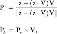
where z is up and V is the view direction.
The effect of applying this transformation to the texture coordinates is that a convex region of the surface will magnify the image behind it, a concave region will shrink the image, and flat (with respect to the viewer) regions will allow rays to pass straight through.
30.4 Conclusion
In this chapter, we hope to have demonstrated that physically based fluid animation is a valuable tool for creating interactive environments, and to have provided some of the basic building blocks needed to start developing a practical implementation. However, this is by no means the end of the line: we have omitted discussion of a large number of possible directions for fluid animation, including melting (Carlson et al. 2002), visco-elastic fluids (Goktekin et al. 2004), and multiphase flows (Lossasso et al. 2006). We have also omitted discussion of a number of interesting data structures and algorithms, such as sparse level sets (Lefohn et al. 2004), which may significantly improve simulation performance; or mesh-based surface extraction (Ziegler et al. 2006), which may permit more efficient rendering of liquids.
30.5 References
Blythe, David. 2006. "The Direct3D 10 System." In ACM Transactions on Graphics (Proceedings of SIGGRAPH 2006) 25(3), pp. 724–734.
Bolz, J., I. Farmer, E. Grinspun, and P. Schröder. 2003. "Sparse Matrix Solvers on the GPU: Conjugate Gradients and Multigrid." In ACM Transactions on Graphics (Proceedings of SIGGRAPH 2003) 22(3), pp. 917–924.
Bridson R., R. Fedkiw, and M. Muller-Fischer. 2006. "Fluid Simulation." SIGGRAPH 2006 Course Notes. In ACM SIGGRAPH 2006 Courses.
Briggs, William L., Van Emden Henson, and Steve F. McCormick. 2000. A Multigrid Tutorial. Society for Industrial and Applied Mathematics.
Carlson, M., P. Mucha, R. Van Horn, and G. Turk. 2002. "Melting and Flowing." In Proceedings of the ACM SIGGRAPH/Eurographics Symposium on Computer Animation.
Fang, S., and H. Chen. 2000. "Hardware Accelerated Voxelization." Computers and Graphics 24(3), pp. 433–442.
Fedkiw, R., J. Stam, and H. W. Jensen. 2001. "Visual Simulation of Smoke." In Proceedings of SIGGRAPH 2001, pp. 15–22.
Foster, N., and R. Fedkiw. 2001. "Practical Animation of Liquids." In Proceedings of SIGGRAPH 2001.
Goktekin, T. G., A.W. Bargteil, and J. F. O'Brien. 2004. "A Method for Animating Viscoelastic Fluids." In ACM Transactions on Graphics (Proceedings of SIGGRAPH 2004) 23(3).
Goodnight, N., C. Woolley, G. Lewin, D. Luebke, and G. Humphreys. 2003. "A Multigrid Solver for Boundary Value Problems Using Programmable Graphics Hardware." In Proceedings of the SIGGRAPH/Eurographics Workshop on Graphics Hardware 2003, pp. 102–111.
Hadwiger, M. 2004. "High-Quality Visualization and Filtering of Textures and Segmented Volume Data on Consumer Graphics Hardware." Ph.D. Thesis.
Hadwiger, M., C. Sigg, H. Scharsach, K. Buhler, and M. Gross. 2005. "Real-time Ray-casting and Advanced Shading of Discrete Isosurfaces." In Proceedings of Eurographics 2005.
Harlow, F., and J. Welch. 1965. "Numerical Calculation of Time-Dependent Viscous Incompressible Flow of Fluid with Free Surface." Physics of Fluids 8, pp. 2182–2189.
Harris, Mark J. 2004. "Fast Fluid Dynamics Simulation on the GPU." In GPU Gems, edited by Randima Fernando, pp. 637–665. Addison-Wesley.
Harris, Mark, William Baxter, Thorsten Scheuermann, and Anselmo Lastra. 2003. "Simulation of Cloud Dynamics on Graphics Hardware." In Proceedings of the SIGGRAPH/Eurographics Workshop on Graphics Hardware 2003, pp. 92–101.
Kass, Michael, Aaron Lefohn, and John Owens. 2006. "Interactive Depth of Field Using Simulated Diffusion on a GPU." Technical report. Pixar Animation Studios. Available online at http://graphics.pixar.com/DepthOfField/paper.pdf.
Krüger, Jens, and Rüdiger Westermann. 2003. "Linear Algebra Operators for GPU Implementation of Numerical Algorithms." In ACM Transactions on Graphics (Proceedings of SIGGRAPH 2003) 22(3), pp. 908–916.
Lefohn, A. E., J. M. Kniss, C. D. Hansen, and R. T. Whitaker. 2004. "A Streaming Narrow-Band Algorithm: Interactive Deformation and Visualization of Level Sets." IEEE Transactions on Visualization and Computer Graphics 10(2).
Li, Wei, Zhe Fan, Xiaoming Wei, and Arie Kaufman. 2005. "Flow Simulation with Complex Boundaries." In GPU Gems 2, edited by Matt Pharr, pp. 747–764. Addison-Wesley.
Liu, Y., X. Liu, and E. Wu. 2004. "Real-Time 3D Fluid Simulation on GPU with Complex Obstacles." Computer Graphics and Applications.
Lossasso, F., T. Shinar, A. Selle, and R. Fedkiw. 2006. "Multiple Interacting Liquids." In ACM Transactions on Graphics (Proceedings of ACM SIGGRAPH 2006) 25(3).
Müller, Matthias, David Charypar, and Markus Gross. 2003. "Particle-Based Fluid Simulation for Interactive Applications." In Proceedings of the 2003 ACM SIGGRAPH/Eurographics Symposium on Computer Animation, pp. 154–159.
Nguyen, D., R. Fedkiw, and H. W. Jensen. 2002. "Physically Based Modeling and Animation of Fire." In ACM Transactions on Graphics (Proceedings of SIGGRAPH 2002) 21(3).
Pharr, Matt, ed. 2005. "Part IV: General-Purpose Computation on GPUs: A Primer." In GPU Gems 2. Addison-Wesley.
Sander, P. V., N. Tatarchuk, and J. Mitchell. 2004. "Explicit Early-Z Culling for Efficient Fluid Flow Simulation and Rendering." ATI Technical Report.
Scharsach, H. 2005. "Advanced GPU Raycasting." In Proceedings of CESCG 2005.
Selle, A., R. Fedkiw, B. Kim, Y. Liu, and J. Rossignac. 2007. "An Unconditionally Stable MacCormack Method." Journal of Scientific Computing (in review). Available online at http://graphics.stanford.edu/~fedkiw/papers/stanford2006-09.pdf.
Sethian, J. A. 1999. Level Set Methods and Fast Marching Methods: Evolving Interfaces in Computational Geometry, Fluid Mechanics, Computer Vision, and Materials Science. Cambridge University Press.
Sigg, Christian, and Markus Hadwiger. 2005. "Fast Third-Order Texture Filtering." In GPU Gems 2, edited by Matt Pharr, pp. 307–329. Addison-Wesley.
Stam, Jos. 1999. "Stable Fluids." In Proceedings of SIGGRAPH 99, pp. 121–128.
Wu, E., Y. Liu, and X. Liu. 2004. "An Improved Study of Real-Time Fluid Simulation on GPU." In Computer Animation and Virtual Worlds 15(3–4), pp. 139–146.
Ziegler, G., A. Trevs, C. Theobalt, and H.-P. Seidel. 2006. "GPU PointList Generation using HistoPyramids." In Proceedings of Vision Modeling & Visualization 2006.
- Contributors
- Foreword
- Part I: Geometry
-
- Chapter 1. Generating Complex Procedural Terrains Using the GPU
- Chapter 2. Animated Crowd Rendering
- Chapter 3. DirectX 10 Blend Shapes: Breaking the Limits
- Chapter 4. Next-Generation SpeedTree Rendering
- Chapter 5. Generic Adaptive Mesh Refinement
- Chapter 6. GPU-Generated Procedural Wind Animations for Trees
- Chapter 7. Point-Based Visualization of Metaballs on a GPU
- Part II: Light and Shadows
-
- Chapter 8. Summed-Area Variance Shadow Maps
- Chapter 9. Interactive Cinematic Relighting with Global Illumination
- Chapter 10. Parallel-Split Shadow Maps on Programmable GPUs
- Chapter 11. Efficient and Robust Shadow Volumes Using Hierarchical Occlusion Culling and Geometry Shaders
- Chapter 12. High-Quality Ambient Occlusion
- Chapter 13. Volumetric Light Scattering as a Post-Process
- Part III: Rendering
-
- Chapter 14. Advanced Techniques for Realistic Real-Time Skin Rendering
- Chapter 15. Playable Universal Capture
- Chapter 16. Vegetation Procedural Animation and Shading in Crysis
- Chapter 17. Robust Multiple Specular Reflections and Refractions
- Chapter 18. Relaxed Cone Stepping for Relief Mapping
- Chapter 19. Deferred Shading in Tabula Rasa
- Chapter 20. GPU-Based Importance Sampling
- Part IV: Image Effects
-
- Chapter 21. True Impostors
- Chapter 22. Baking Normal Maps on the GPU
- Chapter 23. High-Speed, Off-Screen Particles
- Chapter 24. The Importance of Being Linear
- Chapter 25. Rendering Vector Art on the GPU
- Chapter 26. Object Detection by Color: Using the GPU for Real-Time Video Image Processing
- Chapter 27. Motion Blur as a Post-Processing Effect
- Chapter 28. Practical Post-Process Depth of Field
- Part V: Physics Simulation
-
- Chapter 29. Real-Time Rigid Body Simulation on GPUs
- Chapter 30. Real-Time Simulation and Rendering of 3D Fluids
- Chapter 31. Fast N-Body Simulation with CUDA
- Chapter 32. Broad-Phase Collision Detection with CUDA
- Chapter 33. LCP Algorithms for Collision Detection Using CUDA
- Chapter 34. Signed Distance Fields Using Single-Pass GPU Scan Conversion of Tetrahedra
- Chapter 35. Fast Virus Signature Matching on the GPU
- Part VI: GPU Computing
-
- Chapter 36. AES Encryption and Decryption on the GPU
- Chapter 37. Efficient Random Number Generation and Application Using CUDA
- Chapter 38. Imaging Earth's Subsurface Using CUDA
- Chapter 39. Parallel Prefix Sum (Scan) with CUDA
- Chapter 40. Incremental Computation of the Gaussian
- Chapter 41. Using the Geometry Shader for Compact and Variable-Length GPU Feedback
- Preface