GPU Gems 3

GPU Gems 3 is now available for free online!

The CD content, including demos and content, is available on the web and for download.

You can also subscribe to our Developer News Feed to get notifications of new material on the site.

Chapter 29. Real-Time Rigid Body Simulation on GPUs

Takahiro Harada
University of Tokyo

We can easily calculate realistic object motions and produce high-quality computer animations by using physically based simulation. For example, making an animation, by hand, of a falling chess piece is not difficult. However, it is very hard to animate several thousand falling chess pieces, as shown in Figure 29-1.

Figure 29-1 Real-Time Simulation Results of Chess Pieces and Tori

In the case of Figure 29-1, simulation is the only practical solution. Simulation remains computationally expensive, though, so any technique that can speed it up, such as the one we propose in this chapter, is welcome. As for real-time applications such as games, in which a user interacts with objects in the scene, there is no other alternative than simulation because the user interaction is unpredictable. Moreover, real-time applications are much more demanding because the simulation frame rate has to be at least as high as the rendering frame rate.

In this chapter, we describe how we use the tremendous computational power provided by GPUs to accelerate rigid body simulation. Our technique simulates a large number of rigid bodies entirely on the GPU in real time. Section 29.1 outlines our approach and Section 29.2 provides a detailed description of its implementation on the GPU.

Several studies use GPUs to accelerate physically based simulations, such as cellular automata (Owens et al. 2005), Eulerian fluid dynamics (Harris 2004), and cloth simulation (Zeller 2005). A common characteristic of these previous studies is that the connectivity of the simulated elements—either particles or grid cells—does not change during the simulation. However, our technique also works even if the connectivity between elements changes over time. We illustrate this in Section 29.3 by briefly discussing how it can be applied to other kinds of physically based simulations, such as granular materials, fluids, and coupling.

29.1 Introduction

The motion of a rigid body is computed by dividing motion into two parts:—translation and rotation—as shown in Figure 29-2. Translation describes the motion of the center of mass, whereas rotation describes how the rigid body rotates around the center of mass. A detailed explanation can be found in Baraff 1997.

Figure 29-2 Translation and Rotation Parts of a Rigid Body Motion

29.1.1 Translation

The motion of the center of mass is easy to understand because it is the same as the motion of a particle. When a force F acts on a rigid body, this force can cause a variation of its linear momentum P. More precisely, the time derivative of P is equal to F:

Equation 1

We obtain the velocity v of the center of mass from P and the rigid body's mass M, using the following formula:

Equation 2

And the velocity is the time derivative of the position x of the center of mass:

Equation 3

29.1.2 Rotation

A force F that acts at some point of a rigid body that is different from the center of mass can also cause a variation of the rigid body's angular momentum L. This variation depends on the relative position r of the acting point to the center of mass. More precisely, the time derivative of L is the torque that is the cross-product of r and F:

Equation 4

Then the angular velocity w, whose norm is the spinning speed, is derived from the angular momentum L:

Equation 5

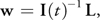
where the 3x3 matrix I(t) is the inertia tensor at time t and I(t)^-1 is its inverse. The inertia tensor is a physical value of a rigid body, which indicates its resistance against rotational motion. Because the inertia tensor changes as the orientation of a rigid body changes, it must be reevaluated at every time step. To calculate I(t)^-1, we have to introduce the rotation matrix R(t), which describes the orientation of a rigid body at time t. The appendix shows how to calculate a rotation matrix from a quaternion. I(t)^-1 is obtained from the rotation matrix at time t as follows:

Equation 6

Now that we have the angular velocity w, the next step is to calculate the time derivative of the rigid body orientation with angular velocity w. There are two ways to store orientation: using a rotation matrix or using a quaternion. We choose to use a quaternion, which is often employed for many reasons. The most important reason is that a rotation matrix accumulates nonrotational motion with time because a matrix represents not only rotation, but also stretch. Therefore, numerical errors that add up during repeated combinations of rotation matrices cause the rigid body to get distorted.

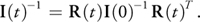
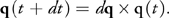
On the other hand, quaternions do not have degrees of freedom for nonrotational motion, and so the rigid body does not get distorted. Also, the quaternion representation is well suited to being implemented on the GPU because it consists of four elements. Thus, it can be stored in the RGBA channels of a pixel. A quaternion q = [s, v_x , v_y , v_z ] represents a rotation of s radians about an axis (v_x , v_y , v_z ). For simplicity, we write it as q = [s, v], where v = (v_x , v_y , v_z ). The variation of quaternion d q with angular velocity w is calculated as the following:

Equation 7

where a = w/|w| is the rotation axis and = |w dt| is the rotation angle.

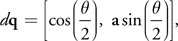
Then the quaternion at time t + dt is updated as follows:

Equation 8

29.1.3 Shape Representation

Now that we know how to calculate rigid body motions, the next step is to compute collision to deal with rigid body interactions. There are several ways to compute collision. In this subsection, we describe a method that is well suited to GPUs and real-time simulation.

In our method, collision detection is based not on the polygons that represent the rigid bodies, but on particles, as done by Bell et al. (2005) and Tanaka et al. (2006). A rigid body is represented by a set of particles that are spheres of identical size, as shown in Figure 29-3. To generate the particles inside a rigid body, we discretize space around the rigid body by defining a 3D grid that encloses it, and we assign one particle for each voxel inside the rigid body. Assuming that the rigid body is represented as a closed mesh, this can be done by casting rays parallel to some axis—usually one of the grid edges—and intersecting them with the mesh. As we progress along a ray, starting from outside the mesh and going from one voxel to the next, we track the number of times the ray intersects the mesh. If this number is odd, we mark each voxel as "inside" the rigid body.

Figure 29-3 Particle Representations of a Chess Piece

The GPU can accelerate this computation—particle generation from a mesh—by using a technique called depth peeling. Depth peeling extracts depth images from 3D objects in depth order (Everitt 2001). When the object is orthographically projected in the direction of the axis, the first depth image extracted by depth peeling contains the depths of the first intersection points of each ray with the mesh (rays enter the mesh at these points). The second depth image contains the depths of the second intersection points of each ray with the mesh (rays exit the mesh at these points), and so on. In other words, odd-numbered depth images contain the depths of the entry points and even-numbered depth images contain the depths of the exit points.

After the extraction, a final rendering pass determines whether or not each voxel is located inside the rigid body. The render target is a flat 3D texture (as described later in Section 29.2.2). The fragment shader (FS) takes a voxel as input and looks up all depth images to determine if the voxel's depth falls between the depth of an odd-numbered image and the depth of an even-numbered image, in that order. If this is the case, the voxel is inside the object. Figure 29-4 illustrates this process.

Figure 29-4 Particle Generation from a Polygon Model by Using Depth Peeling

29.1.4 Collision Detection

Because we represent a rigid body as a set of particles, collision detection between rigid bodies with complicated shapes means we simply need to detect collisions between particles. When the distance between two particles is smaller than their diameter, collision occurs. A benefit of this particle representation is the controllability of simulation speed and accuracy. Increasing the resolution of particles increases computation cost—however, we get a more accurate representation of the shape and the accuracy of the simulation improves. Therefore, we can adjust the resolution, depending on the purpose. For example, for real-time applications where computation speed is important, we can lower the resolution.

However, the particle representation involves a larger number of elements, whose collisions must all be computed. If we employ a brute-force strategy, we have to check n ² pairs for n particles. This approach is impractical, plus it is difficult to solve such a large problem in real time even with current GPUs. Thus, we use a three-dimensional uniform grid to reduce the computational burden. The grid covers the whole computational domain, and the domain is divided into voxels. The voxel index g = (g_x , g_y , g_z ) of a particle at p = (p_x , p_y , p_z ) is calculated as follows:

Equation 9

where s = (s_x , s_y , s_z ) is the grid corner with smallest coordinates and d is the side length of a voxel.

Then the particle index is stored in the voxel to which the particle belongs, as shown in Figure 29-8. With the grid, particles that collide with particle i are restricted to (a) the particles whose indices are stored in the voxel that holds the index of particle i and (b) the 26 voxels adjacent to (that is, surrounding) the voxel that holds the index of particle i. The maximum number of particles stored in a voxel is finite (four particles in our implementation) because the interparticle forces work to keep the distance between particles equal to their diameter, as described later in Section 29.2.4. Consequently, the efficiency is improved from O(n ²) to O(n). Computation becomes most efficient when the side length of a voxel is set to the diameter of particles, because the number of voxels we have to search is the smallest: 3² in two dimensions and 3³ in three dimensions.

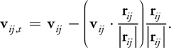
29.1.5 Collision Reaction

The interparticle forces between colliding pairs are calculated by applying the discrete element method (DEM), which is a method for simulating granular materials (Mishra 2003). A repulsive force f _i _, _s , modeled by a linear spring, and a damping force f _i _, _d , modeled by a dashpot—which dissipates energy between particles—are calculated for a particle i colliding with a particle j as the following:

Equation 10

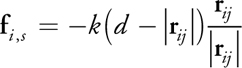
Equation 11

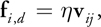
where k, , d, r _ij , and v _ij are the spring coefficient, damping coefficient, particle diameter, and relative position and velocity of particle j with respect to particle i, respectively. A shear force f _{i, t} is also modeled as a force proportional to the relative tangential velocity v _ij _, _t :

Equation 12

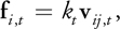
where the relative tangential velocity is calculated as

Equation 13

Then the force and torque applied to a rigid body are the sums of the forces exerted on all particles of the rigid body:

Equation 14

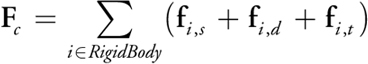
Equation 15

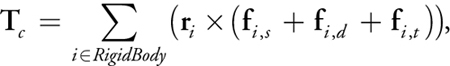
where r _i is the current relative position of particle i to the center of mass.

29.2 Rigid Body Simulation on the GPU

29.2.1 Overview

So far we have described the basic algorithm of rigid body simulation. In this section we explain how to implement this simulation on the GPU.

An iteration consists of the following five stages, which are shown in the flow chart in Figure 29-5.

Figure 29-5 Flow Chart of Rigid Body Simulation on the GPU

Computation of particle values
Grid generation
Collision detection and reaction
Computation of momenta
Computation of position and quaternion

We do not describe basic GPGPU techniques; readers unfamiliar with these techniques can refer to references such as Harris 2004 and Harris 2005.

29.2.2 The Data Structure

To simulate rigid body motion on the GPU, we must store all the physical values for each rigid body as textures. The physical values can be stored in a 1D texture, but a 2D texture is often used because current GPUs have restrictions on the size of 1D textures.

An index is assigned to each rigid body. To store the physical values of each rigid body in a 2D texture, this index is converted to a 2D index and then the texture coordinates are calculated from the 2D index. Figure 29-6 illustrates this process. Each value of a rigid body is stored in the texel at the texture coordinates. For rigid bodies, we prepare textures for linear and angular momenta, position, and the orientation quaternion. Two textures are prepared for each value because they are updated by reading from one texture and then writing to the other texture.

Figure 29-6 Data Structures of the Physical Values of Rigid Bodies and Their Particles

We also need textures for the values of the particle's position, velocity, and relative position to the center of mass. If a rigid body consists of four particles, we need a texture four times larger than the textures of rigid bodies. The size of the textures is adjusted, depending on the number of particles that belong to a rigid body. The indices of the particles that belong to a rigid body are calculated from the rigid body index. As with the rigid body index, a particle index is converted into 2D texture coordinates (as shown in Figure 29-6). Because these particle values are dynamically derived from the physical values of rigid bodies, only one texture is enough to store each.

In addition to storing physical values, we need to allocate memory for the uniform grid on the GPU, which is the data structure that helps us search neighboring particles. We use a data layout called a flat 3D texture, in which the 3D grid is divided into a set of 2D grids arranged into a large 2D texture (Harris et al. 2003). We arrange the grid this way because GPUs did not support writing to slices of a 3D texture at the time of implementation. The NVIDIA GeForce 8 Series supports it, but there can still be performance advantages in using 2D textures.

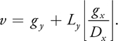
To read and write a value in a grid, we need to convert the 3D grid coordinates to the 2D texture coordinates. Let the size of a 3D grid be L_x x L_y x L_z and the number of 2D grids in the 2D texture be D_x x D_y , as shown in Figure 29-7. The 2D texture coordinates (u, v) are calculated from the 3D grid coordinates (g_x , g_y , g_z ) as follows:

Equation 16

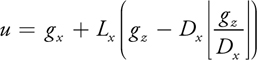
Equation 17

Figure 29-7 A Flat 3D Texture

29.2.3 Step 1: Computation of Particle Values

Most of the following operations use the physical values of particles, so we should compute them first. The current relative position r _i of a particle i to the center of mass of rigid body j is derived from current quaternion Q j and the initial relative position r _i ⁰ of particle i:

Equation 18

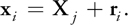
Then the particle position x _i is computed from the position of the center of mass X _j and the relative position of the particle r _i as follows:

Equation 19

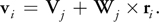
Particle velocity v _i is also computed with velocity V _j and angular velocity W _j of the rigid body as follows:

Equation 20

Storing the current relative positions of particles to a texture is necessary for some of the following steps of our simulation.

29.2.4 Step 2: Grid Generation

In this step we generate the uniform grid data structure. For each particle, we store the particle index at the pixel that corresponds to the voxel where the particle belongs. This operation cannot be performed in a fragment shader because it is a scattering operation (Buck 2005). Instead, we use a vertex shader (VS), which can write a value to an arbitrary position by rendering a vertex as a point primitive of size 1.

We prepare and assign vertices to each particle. In the VS, the particle position is read from the particle position texture, and the voxel index is calculated with Equation 9. Then the coordinates in the grid texture are calculated from the voxel index (as described in Section 29.2.2), the vertex position is set to the grid coordinates, and the color is set to the particle index. However, when we use this simple method, the grid is usually not generated correctly, because only one value is stored per pixel. Consequently, when there are several particles in a voxel, the procedure fails.

To solve this problem, we use a method—described in the following paragraph—that allows us to store, at most, four particles per voxel. Four particles per voxel is enough if the side length of a voxel is smaller than the particle diameter, and if the particles do not interpenetrate—which is our scenario because there is repulsive force between the particles. We set the side length of a voxel equal to the particle diameter; we noticed that overflow rarely occurs.

The method we use is similar to the stencil routing technique used by Purcell et al. (2003), but our method does not have to prepare complicated stencil patterns at every iteration. We prepare the vertices and arrange them, in advance, in ascending order of particle indices. Then, let us assume that there are four particles ending up in a voxel whose indices are p ₀, p ₁, p ₂, and p ₃, arranged in ascending order and rendered in this order. Our goal is to store these values, respectively, into the RGBA channels of a pixel, as shown in Figure 29-8, and we achieve this in four rendering passes. During each pass, we render all the vertices by using the VS described earlier, and then the FS outputs the particle index to the color as well as to the depth of the fragment. Using depth test, stencil test, and color masks, we select which index and channels to write to.

Figure 29-8 A Grid and Particle Indices in the Grid Texture

In the first pass, we want to write p ₀ to the R channel. The vertex corresponding to p ₀ has the smallest depth value among the four vertices, so we clear the depth of the buffer to the maximum value and set the depth test to pass smaller values. In the second pass, we want to write p ₁ to the G channel. We do this by first setting the color mask so that the R channel is not overwritten during this pass. Then we use the same depth buffer as in the first pass without clearing it, and set the depth test to pass larger values. So p ₀ will fail the depth test, but p ₁, p ₂, and p ₃ will not. To write only p ₁, we make p ₂ and p ₃ fail the stencil test by clearing the stencil buffer before rendering to zero, setting the stencil function to increment on depth pass, and setting the stencil test to fail when the stencil value is larger than one. This approach works because p ₁ is rendered before p ₂ and p ₃. The settings of the third and fourth passes are identical to the settings of the second pass, except for the color mask. The RGA and RGB channels are masked in these two last passes, respectively. Also, the same depth buffer is used but never cleared, and the stencil buffer is used and cleared to zero before each pass. The pseudocode of grid generation is provided in Listing 29-1.

This method could be extended to store more than four particles per voxel by rendering to multiple render targets (MRTs).

Example 29-1. Pseudocode of Grid Generation

    //=== 1 PASS colorMask(GBA); depthTest(less); renderVertices(); //===2 PASS colorMask(RBA); depthTest(greater); stencilTest(greater, 1); stencilFunction(increment); clear(stencilBuffer); renderVertices(); //=== 3 PASS colorMask(RGA); clear(stencilBuffer); renderVertices(); //=== 4 PASS colorMask(RGB); clear(stencilBuffer); renderVertices();

29.2.5 Step 3: Collision Detection and Reaction

Particles that can collide with other particles are limited to colliding with the particles whose indices are stored (a) in the voxel of the uniform grid to which the particle belongs and (b) in the adjacent voxels, for a total of 3 x 3 x 3 = 27 voxels. To detect the collisions of particle i, first we derive the grid coordinates of the particle from the position of particle i. Then indices stored in the 27 voxels are looked up from the grid texture. We detect collisions by calculating the distance of particle i to these particles.

We do not need to divide collision detection into broad and narrow phases in this collision detection technique. All we have to do is to compute a simple particle-particle distance. After collision is detected, the reaction forces between particles are calculated with Equations 10, 11, and 12. The computed collision force is written to the particle force texture. The collision detection and reaction can be executed in a single shader. The pseudocode is provided in Listing 29-2.

Example 29-2. Pseudocode of Collision Detection and Reaction

 gridCoordinate=calculateGridCoordinate(iParticlePosition); FOREACH of the 27 voxels   jIndex = tex2D(gridTexture, gridCoordinate);   FOREACH RGBA channel C of jIndex     jParticlePosition = tex2D(positionTexture, index2TexCrd(C));     force += collision(iParticlePosition, jParticlePosition);   END FOR END FOR

29.2.6 Step 4: Computation of Momenta

After calculating the forces on particles, we use Equations 1 and 4 to compute momenta. Computing linear momentum variation of a rigid body requires adding up the forces that act on the particles that belong to the rigid body. This operation is done in a single fragment shader that is invoked once per rigid body. The FS reads the forces from the particle force texture and writes the calculated value to the linear momentum texture. If the number of particles per rigid body is large, we might be able to implement this sum more efficiently as a parallel reduction in multiple passes.

Similarly, computing the angular momentum variation requires the relative positions of particles to the center of mass, but these positions have already been computed in a previous step and stored in a texture. It is convenient to execute both computations in the same shader and output the results in multiple render targets, as shown in Listing 29-3.

Example 29-3. Pseudocode for the Computation of Momenta

 FOR all particles belonging to a rigid body   particleIndex = particleStartIndex + i;   particleTexCoord = particleIndex2TexCoord(particleIndex);   linearMomentum += tex2D(forceOnParticle, particleTexCrd);   angularMomentum += cross(tex2D(relativePosition, particleTexCrd),   tex2D(forceOnParticle, particleTexCrd)); END FOR

29.2.7 Step 5: Computation of Position and Quaternion

Now that we have the current momenta in a texel assigned to each rigid body, we perform the position and quaternion updates like any other standard GPGPU operation.

The momenta and its previous position and quaternion are read from the texture, and the updated position and quaternion are calculated using Equations 3 and 8. This operation can also be performed in a single shader with MRTs.

29.2.8 Rendering

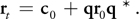
Each rigid body is associated with a polygon model and rendered using the position c ₀ of the center of mass and quaternion q, calculated in Section 29.2.7. The vertex shader reads c ₀ and q from textures based on the texture coordinates derived from the rigid body index, and then the current position of vertex r _t is calculated from the unrotated relative vertex position r ₀ as follows:

Equation 21

29.2.9 Performance

We have implemented the present method on an NVIDIA GeForce 8800 GTX and tested several scenes. In Figure 29-1, 16,384 chess pieces and 10,922 tori are dropped. In both simulations, 65,536 particles are used, and the simulations run at 168 iterations per second (ips) and 152 ips, respectively. When we render the scene at every iteration, the frame rates drop to 44 frames per second (fps) and 68 fps, respectively.

Figure 29-9 shows the results with rigid bodies that have much more complicated shapes: 963 bunnies and 329 teapots. The bunny consists of 68 particles, and the teapot consists of 199 particles. The total number of rigid particles is about 65,000 in these scenes. These simulations run at 112 ips and 101 ips, respectively. The particle representations used in these simulations are solid (that is, the inside of the model is filled with particles). If the particles are placed only on the surface, the simulation can be sped up and still work well. There are 55 particles on the surface of the bunny and 131 particles on the surface of the teapot. With the same number of rigid bodies but a smaller number of rigid particles, the simulations run at 133 ips and 148 ips, respectively. In all these rigid body simulations, the size of the uniform grid is 128³.

Figure 29-9 Simulation Results of 963 Bunnies and 329 Teapots

Note that for large computational domains, a uniform grid is not the best choice for storing particle indices for rigid bodies. Rigid bodies do not distribute over the computational domain uniformly; therefore, many voxels contain no particle indices and graphics memory is wasted. In these cases, we would require a more efficient data structure—one that is dynamic, because the distribution of objects changes during the simulation.

29.3 Applications

As mentioned earlier, our technique works even if the connectivity between elements changes over time. The rigid body simulation explained in this chapter is an example of such a simulation in which the connectivity dynamically changes. In this section, we briefly discuss how it can be applied to other kinds of physically based simulations, such as granular materials, fluids, and coupling.

29.3.1 Granular Materials

The rigid body simulator presented in this chapter can be easily converted to a granular material simulator because the method used to compute the collision reaction force is based on the discrete element method, which has been developed for simulation of granular materials (Mishra 2003). Instead of using particle forces to update the momenta of rigid bodies, we use the particle forces to directly update the positions of the particles. Figure 29-10 (left) shows a result of the simulation. The simulation with 16,384 particles runs at about 285 ips.

Figure 29-10 Particle-Based Simulations on GPUs

29.3.2 Fluids

The rigid body simulator presented in this chapter can also be applied to fluid simulation. The momentum conservation equation of fluids is this:

Equation 22

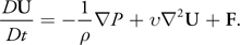
We employ a particle-based method that discretizes fluids to a set of particles and solves the equation by calculating particle interaction forces. Smoothed particle hydrodynamics(SPH) is a particle-based method often used in computer graphics (details can be found in Müller et al. 2003). A physical value at particle position is calculated as a weighted sum of the values of neighboring particles. Therefore, we have to search for neighboring particles. The difficulty in implementing SPH on the GPU is that the neighborhood relationship among particles dynamically changes during the simulation (in other words, the connectivity among particles is not fixed).

Now that we know a way to generate a uniform grid on the GPU, we can search for neighboring particles dynamically. Although we search for neighboring particles once per iteration in the rigid body simulation, in the SPH simulation we have to search twice. First, we have to search for neighboring particles to compute the density. Then, the pressure force is derived from the densities of neighboring particles. Therefore, the computational cost is higher than for the rigid body simulation. However, we can obtain unprecedented performance with the GeForce 8800 GTX, as shown in Figure 29-10 (right). Here the particle positions are output to files, and then the fluid surface constructed from them, using marching cubes, is rendered by an offline renderer (Lorensen and Cline 1987). The simulation uses 1,048,576 fluid particles, with a uniform grid whose size is 256³ and whose speed is about 1.2 ips. The speed is not fast enough for real-time applications, but a simulation with a few tens of thousands of fluid particles runs at about 60 frames/sec. Besides using this simulation for a real-time application, we can use it to accelerate offline simulations for high-quality animation productions and more. Finally, we are limited on the number of particles we can use because of the size of the GPU memory. With 768 MB of video memory, we can use up to about 4,000,000 fluid particles.

29.3.3 Coupling

We can use GPUs to accelerate not only a simple simulation, but also simulations in which several simulations are interacting with each other. The particle representation of rigid bodies described in this chapter makes it easy to couple it with particle-based fluid simulations. Figure 29-11 (top) shows a fluid simulation coupled with a rigid body simulation. The interaction forces are computed by treating particles belonging to rigid bodies as fluid particles and then using the forces to update the momenta of rigid bodies. Glasses are stacked and fluid is poured in from the top. After that, another glass is thrown into the stack. This simulation uses 49,153 fluid particles and runs at about 18 ips.

Figure 29-11 Coupling of Simulations

The techniques are not limited to particle-based simulations. In Figure 29-11 (bottom), we show the results of coupling particle-based fluid simulation and cloth simulation. We see that a mesh-based simulation can be integrated with a particle-based fluid simulation as well. Both the cloth and the fluid simulations are performed on the GPU, and the interaction is also computed on it. The simulations run at about 12 ips with 65,536 fluid particles, and each piece of cloth consists of 8,192 polygons. Videos of both simulations are available on this book's accompanying DVD.

29.4 Conclusion

In this chapter we have described techniques for implementing rigid body simulation entirely on the GPU. By exploiting the computational power of GPUs, we simulate a large number of rigid bodies, which was previously difficult to perform in real time. We showed that the present technique is applicable not only to rigid body simulation but also to several other kinds of simulations, such as fluids.

There is room for improving the accuracy of the rigid body simulation. For example, we could use the present particle-based collision detection technique as the broad phase and implement a more accurate method for the narrow phase.

We are sure that what we have shown in the application section is just a fraction of what is possible, and we hope that others will explore the possibility of GPU physics by extending the present techniques.

29.5 Appendix

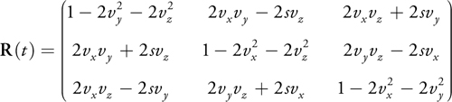
Rotation matrix R(t) is calculated with quaternion q = [s, v_x , v_y , v_z ]:

The multiplication of quaternions q ₀ = [s ₀, v ₀] and q ₁ = [s ₁, v ₁] is

q ₀ x q ₁ = [s ₀ s ₁ - v ₀. v ₁, s ₀ v ₁ + s ₁ v ₀ + v ₀ x v ₁].

29.6 References

Baraff, David. 1997. "An Introduction to Physically Based Modeling: Rigid Body Simulation 1—Unconstrained Rigid Body Dynamics." SIGGRAPH '97 Course Notes.

Bell, Nathan, Yizhou Yu, and Peter J. Mucha. 2005. "Particle-Based Simulation of Granular Materials." In Proceedings of the ACM SIGGRAPH/Eurographics Symposium on Computer Animation, pp. 77–86.

Buck, Ian. 2005. "Taking the Plunge into GPU Computing." In GPU Gems 2, edited by Matt Pharr, pp. 509–519. Addison-Wesley.

Everitt, Cass. 2001. "Interactive Order-Independent Transparency." NVIDIA technical report. Available online at http://developer.nvidia.com/object/Interactive_Order_Transparency.html.

Harris, Mark J. 2004. "Fast Fluid Dynamics Simulation on the GPU." In GPU Gems, edited by Randima Fernando, pp. 637–665. Addison-Wesley.

Harris, Mark. 2005. "Mapping Computational Concepts to GPUs." In GPU Gems 2, edited by Matt Pharr, pp. 493–508. Addison-Wesley.

Harris, Mark, William Baxter, Thorsten Scheuermann, and Anselmo Lastra. 2003. "Simulation of Cloud Dynamics on Graphics Hardware." In Proceedings of the SIGGRAPH/Eurographics Workshop on Graphics Hardware 2003, pp. 92–101.

Lorensen, William E., and Harvey E. Cline. 1987. "Marching Cubes: A High Resolution 3D Surface Construction Algorithm." In Proceedings of the 14th Annual Conference on Computer Graphics and Interactive Techniques, pp. 163–169.

Mishra, B. K. 2003. "A Review of Computer Simulation of Tumbling Mills by the Discrete Element Method: Part 1—Contact Mechanics." International Journal of Mineral Processing 71(1), pp. 73–93.

Müller, Matthias, David Charypar, and Markus Gross. 2003. "Particle-Based Fluid Simulation for Interactive Applications." In Proceedings of the 2003 ACM SIGGRAPH/Eurographics Symposium on Computer Animation, pp. 154–159.

Owens, John, David Luebke, Naga Govindaraju, Mark Harris, Jens Krüger, Aaron Lefohn, and Timothy Purcell. 2005. "A Survey of General-Purpose Computation on Graphics Hardware." In Proceedings of Eurographics 2005, State of the Art Reports, pp. 21–51.

Purcell, Timothy J., Craig Donner, Mike Cammarano, Henrik-Wann Jensen, and Pat Hanrahan. 2003. "Photon Mapping on Programmable Graphics Hardware." In Proceedings of the SIGGRAPH/Eurographics Workshop on Graphics Hardware 2003, pp. 41–50.

Tanaka, Masayuki, Mikio Sakai, and Seiichi Koshizuka. 2006. "Rigid Body Simulation Using a Particle Method." In ACM SIGGRAPH Research Posters, no. 132.

Zeller, Cyril. 2005. "Cloth Simulation on the GPU." In ACM SIGGRAPH Sketches, no. 39.

The author would like to thank to Seiichi Koshizuka and Masayuki Tanaka for valuable advice and discussion.

Part II: Light and Shadows

Part III: Rendering

Part IV: Image Effects

Part V: Physics Simulation

Part VI: GPU Computing

Preface