GPU Gems 3

GPU Gems 3 is now available for free online!

The CD content, including demos and content, is available on the web and for download.

You can also subscribe to our Developer News Feed to get notifications of new material on the site.

Chapter 26. Object Detection by Color: Using the GPU for Real-Time Video Image Processing

Ralph Brunner
Apple

Frank Doepke
Apple

Bunny Laden
Apple

In this chapter, we describe a GPU-based technique for finding the location of a uniquely colored object in a scene and then utilizing that position information for video effects. The technique uses a pixel shader in an atypical manner: to calculate a centroid and area rather than a per-pixel effect.

Object detection and tracking have applications in robotics, surveillance, and other fields. As the number of consumers who own computers equipped with video cameras increases, so do the possibilities of using the GPU for tracking objects for games and to enable new user-interaction models. In this chapter, we discuss one use of object detection: overlaying a tracked object with an image. As you'll see, the computational requirements of this implementation are so low that we can process the entire image area every video frame; we don't need to use any sophisticated region-of-interest tracking methods. By using the GPU for centroid computation, we leave the CPU free for other tasks, such as video decoding and encoding.

Because our program uses the Core Image image-processing framework on Mac OS X, we begin the chapter with a brief description of Core Image, why we use it, and how it works. Next we provide an overview of tracking objects using color, and then we describe the computations and kernel routines that process the video image.

26.1 Image Processing Abstracted

Core Image is an image-processing framework built into Mac OS X. It uses the GPU to perform real-time, pixel-accurate image processing. We chose to use Core Image to tackle the object detection and tracking problem rather than a kernel-level technology because Core Image does the following:

Abstracts the low-level work performed by the GPU in an easy-to-use, high-level programming interface. You can easily follow and adapt the technique described in this chapter without needing to learn the low-level implementation details of specific hardware. Core Image takes care of all hardware-specific optimizations for you. It also converts image formats when necessary.
Processes only when necessary. Because Core Image is predicated upon laziness, it is extremely efficient. It does not process data unless it must, and when it does, it takes the easiest route possible. When you apply a filter to an image, Core Image processes the pixels only when you need to paint the pixels to a destination. If you apply several filters in sequence, Core Image may change the order of processing or merge operations to perform the processing as optimally as possible.

We use Core Image to build several custom filters for the object-tracking problem. Before you read the specifics, you'll want to get an overall idea of the processing path, the components of a Core Image filter, and the terminology.

The custom Core Image filters that we use for object tracking have an Objective-C portion and a C portion. The Objective-C portion of a Core Image filter performs all the high-level tasks needed for image processing and calls the low-level routines that operate on pixels. A filter produces an output image by carrying out these steps:

Setting up one or more objects, called samplers, to fetch pixels from the source image. If necessary, a sampler can apply a transform to the pixel prior to handing off the pixel for processing.
Applying kernel routines to operate on the pixels supplied by the sampler. A kernel routine performs per-pixel processing. It always produces a four-element vector as output. Usually the vector represents RGBA (red, green, blue, alpha), but as you'll see in this chapter, that's not always the case. A filter can apply one or more kernel routines in sequence, or it can repeatedly apply the same kernel. Filters that apply more than one kernel routine are multipass filters.
Writing the resulting image to a destination, most typically the screen.

The C portion of a Core Image filter includes the kernel routines that perform per-pixel processing on the GPU. The kernel routines use the Core Image kernel language, which is an extension to OpenGL Shading Language. This extension defines functions, data types, and keywords that make it easy to specify image-processing operations. You can use Core Image kernel language symbols together with the subset of the OpenGL Shading Language routines that Core Image supports.

You won't see the code for the Objective-C portion in this chapter; it's in the sample on the DVD that accompanies this book. What you will see in this chapter is code for most of the kernel routines that make up the C portion of the Core Image filter.

Now that you know a bit about what makes up a Core Image filter, let's take a look at how Core Image processes an image. See Figure 26-1 for an illustration of the process. The filter assembles the source image (or images) and then sets up a sampler for each source, defining any transformation that the sampler might need to perform after it fetches a pixel from a source. Setting up the sampler is straightforward; most of the time it involves creating and naming a sampler object and attaching it to an image source. Next the filter calls a routine to apply a kernel, passing the following:

The name of the kernel routine to apply.
The sampler (or samplers) needed by the kernel.
A list of the arguments needed by the kernel.
A dictionary (key-value pairs) of options that controls how Core Image evaluates the kernel. For example, you might want to specify the size of the output image.

Figure 26-1 The Pixel Processing Path in Core Image

When applying a kernel, Core Image sets up a calculation path that begins at the destination and works its way back to the source. Although this might seem a bit backward, this looking-ahead behavior is quite efficient because it allows Core Image to limit the processing to those pixels that are required to compute the final result. Take a look at Figure 26-1, and you'll see that the only pixels that need processing are those that overlap in the two source images. By looking ahead, Core Image figures a domain of definition: the area outside of which all pixels are transparent. There is no need to process any pixel that won't be seen. The alternative to looking ahead is to process every pixel and then, at the end, eliminate those that aren't needed.

The shaded area in each of the source images in Figure 26-1 is the region of interest (ROI). The ROI defines the area in the source image from which a sampler takes pixel information to provide to the kernel for processing. The way the ROI and the domain of definition relate to each other determines whether the filter needs to perform additional setup work prior to applying a kernel. The ROI and the domain of definition can relate in these ways:

They can coincide exactly: there is a 1:1 mapping between source and destination. For example, a hue filter processes a pixel from the working-space coordinate (r, s) in the ROI to produce a pixel at the working-space coordinate (r, s) in the domain of definition.
They can depend on each other, but be modulated in some way. Some of the most interesting filters—blur and distortion, for example—use many source pixels in the calculation of one destination pixel. For example, a distortion filter might use a pixel (r, s) and its neighbors from the working coordinate space in the ROI to produce a single pixel (r, s) in the domain of definition.
They can be independent. In this case, the domain of definition is calculated from values in a lookup table that are provided by the sampler. The locations of values in the map or table are unrelated to the working-space coordinates in the source image and the destination. A value located at (r, s) in a shading image does not need to be the value that produces a pixel at the working-space coordinate (r, s) in the domain of definition. Many filters use values provided in a shading image or lookup table in combination with an image source. For example, a color ramp or a table that approximates a function, such as the arcsin() function, provides values that are unrelated to the notion of working coordinates.

Core Image assumes that the ROI and domain of definition coincide unless you tell it otherwise. The object-tracking problem requires some filters for which we need to define a region of interest.

26.2 Object Detection by Color

If you've ever watched the audience at a tennis match, you know exactly what color tracking is. As the green tennis ball flies from side to side of the court, the heads of the onlookers move side to side. In this section, you'll see how to process video input of a moving ball and overlay the ball with an image of a duck, as shown in Figure 26-2. We process 1280x720 video in real time (30 frames per second) on a Macintosh computer equipped with an NVIDIA GeForce 7300 GT graphics card.

Figure 26-2 From Ball Tossing to Duck Tossing

As illustrated in Figure 26-3, these are the tasks needed to detect an object using color and then track it:

Create a masking image by comparing each pixel with a target color value. Convert pixels that fall within the range to white, and convert those that fall outside the range to black.
Find the centroid of the target color. The centroid of the tracked color defines the center position for the overlay image. We use a multipass pixel-processing kernel to compute a location. The output of this phase is a 1x1-pixel image, containing the coordinate of the centroid in the first two components (pixel.rg) and the area in the third component (pixel.b). We use the area later to estimate the distance of the object from the camera.
Composite an image over the detected object. Assuming the shape of the object does not change with respect to the frame, then the change in area of the tracked color is proportional to the square of the distance of the object from the viewer. We use this information to scale the overlay image, so that the overlay image increases or decreases in size appropriately. (The assumption doesn't hold for objects such as an expanding balloon or an expanding pool of liquid, but it works well for the spherical ball in our sample.)

Figure 26-3 The Tasks Needed to Track Color

We discuss each task in more detail in the following sections.

26.2.1 Creating the Mask

We create the mask using a Mask from Color filter that has two input parameters: an input color and an input threshold. The input color defines the color to track. The input threshold defines the range of color values around the input color that are included in the calculations for tracking, as shown in Figure 26-4. Choosing the threshold is a bit of an art. You'll want to make sure it is small enough to avoid extraneous noise (as you'll see in Figure 26-5, upcoming) but large enough to allow for lighting variations in the color of the object that you want to track. Recall that a Core Image filter (in this case, Mask from Color) performs the high-level tasks of setting up samplers and applying a kernel routine.

Figure 26-4 Targeting the Colors

Figure 26-5 The Masked Image

The Mask from Color filter calls the maskFromColor() kernel routine shown in Listing 26-1 to compute the mask. Before we get into describing this kernel routine in more detail, let's review the keywords in the Core Image kernel language that we use in Listing 26-1, starting with two data types: sampler and __color. We described samplers earlier; the sampler keyword specifies an object that fetches samples from a source image (or, if appropriate, a lookup table.) The __color data type specifies a vector of color values that Core Image must match to the current working color space.

The kernel keyword tags a kernel routine; it is placed before the return type, which is always a vec4 data type. All parameters to a kernel routine are implicitly marked uniform. You cannot mark parameters out and inout; it's not allowed.

The listing contains several functions that are specific to the Core Image kernel language. The samplerCoord() function returns the position (a two-element vector) in sampler space of the current pixel. It takes care of all the coordinate mapping from the source to the working coordinate space (such as rotating and scaling). The sample() function returns the pixel value produced from the sampler at the given position, where the position is given in sampler space.

Example 26-1. Routines Used by the Color Masking Filter

    vec3 normalizeColor(vec3 color ) {   return color / max(dot(color, vec3(1.0/3.0)), 0.001); } kernel vec4 maskFromColor(sampler image, __color color,                           float threshold) {   float d;   vec4 p;   // Compute distance between current pixel color and reference color.   p = sample(image, samplerCoord(image));   d = distance(normalizeColor(p.rgb), normalizeColor(color.rgb));   // If color difference is larger than threshold, return black.    return (d > threshold) ? vec4(0.0) : vec4(1.0); }

Prior to calling the maskFromColor() kernel routine shown in Listing 26-1, the Mask from Color filter creates and sets up a sampler object to fetch pixels from the video input image. Then it passes the sampler object, the target color, and a threshold value to the maskFromColor() kernel routine. The kernel routine normalizes the color values to compensate for variations in the shading of the object due to lighting conditions. The kernel then calculates the distance between the color of the current pixel and the target color. If the color value is less than the threshold, the kernel routine returns (1.0, 1.0, 1.0, 1.0). Otherwise, it returns (0.0, 0.0, 0.0, 0.0). The mask returned for the input image shown in Figure 26-2 is shown in Figure 26-5.

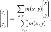
26.2.2 Finding the Centroid

We compute the centroid of the masked area as a weighted average of all the coordinates in the mask image. If m(x, y) is the value of the mask image at coordinate (x, y), the equation to compute the centroid is

Equation 1

Our implementation, the coordinateMask() kernel routine shown in Listing 26-2, first creates an image that contains these three components:

(x · m(x, y),

y · m(x, y),

m(x, y)).

The routine uses the Core Image kernel language function destCoord(), which returns the position, in working-space coordinates, of the pixel we are currently computing.

Example 26-2. A Routine That Creates a Mask

    kernel vec4 coordinateMask(sampler mask, vec2 invSize) {   vec4 d;   // Create a vector with (x,y, 1,1), normalizing the coordinates    // to 0-1 range.   d = vec4(destCoord()*invSize, vec2(1.0));   // Return this vector weighted by the mask value    return sample(mask, samplerCoord(mask))*d; }

Note that if we were to sum the values of all the pixel values computed by the coordinateMask() kernel routine, the first two components of the result would correspond to the numerator of Equation 1, while the third component would correspond to the denominator of that equation. Instead of computing the sum, our implementation computes the mean value over all those pixels and then multiplies (scales) by the number of pixels to get the sum.

We compute the average value of the image by repeatedly downsampling the image, from one that is nxn pixels to one that is 1x1 pixel, as shown in Figure 26-6.

Figure 26-6 Downsampling an Image to Compute the Mean Pixel Value

We downsample by a factor of four, both horizontally and vertically, in a single pass, using the scaleXY4() kernel routine shown in Listing 26-3. Note that there are only four sample instructions in this routine to gather the values for 16 pixels. Requesting the texel between the sample locations leverages the linear interpolation hardware, which fetches the average of a 2x2-pixel block in a single operation.

Example 26-3. A Routine That Downsamples by a Factor of Four

    kernel vec4 scaleXY4(sampler image) {   vec4 p0,p1,p2,p3;   vec2 d;   // Fetch the position of the coordinate we want to compute,    // scale it by 4.   d = 4.0*destCoord();   // Fetch the pixels that surround the current pixel.   p0 = sample(image, samplerTransform(image, d + vec2(-1.0,-1.0)));   p1 = sample(image, samplerTransform(image, d + vec2(+1.0,-1.0)));   p2 = sample(image, samplerTransform(image, d + vec2(-1.0,+1.0)));   p3 = sample(image, samplerTransform(image, d + vec2(+1.0,+1.0)));   // Sum the fetched pixels, scale by 0.25.    return 0.25*(p0 + p1 + p2 + p3); }

The samplerTransform() function is another Core Image kernel language function. It returns the position in the coordinate space of the source (the first argument) that is associated with the position defined in working-space coordinates (the second argument).

If the image is not square, you won't end up with a 1x1 image. If that's the case, you will need to downsample by a factor of two in the horizontal or vertical direction until the result is reduced to a single pixel.

If the width or height of the image is not a power of two, this method computes the mean over an area larger than the actual image. Because the image is zero outside its domain of definition, the result is simply off by a constant factor: the image area divided by the downsampled area. The implementation we provide uses the Core Image built-in filter CIColorMatrix filter to scale the result appropriately, so that the filter works correctly for any image size.

At the end of the downsampling passes, we use the centroid() kernel routine shown in Listing 26-4 to perform a division operation to get the centroid. The output of this phase is a 1x1-pixel image that contains the coordinate of the centroid in the first two components (pixel.rg) and the area in the third component (pixel.b).

Example 26-4. A Kernel Routine Whose Output Is a Centroid and an Area

    kernel vec4 centroid(sampler image) {   vec4 p;   p = sample(image, samplerCoord(image));   p.xy = p.xy / max(p.z, 0.001);   return p; }

26.2.3 Compositing an Image over the Input Signal

To illustrate the result of the centroid calculation, we composite an image (in this case, a duck) on top of the video signal, using the duckComposite kernel routine shown in Listing 26-5. We also scale the composited image according to a distance estimate, which is simply the square root of the area from the previous phase. Note that Core Image, by default, stores image data with premultiplied alpha. That makes the compositing in this case simple (see the last line in Listing 26-5).

Example 26-5. A Kernel Routine That Overlays an Image

    kernel vec4 duckComposite(sampler image, sampler duck,                           sampler location, vec2 size,                           vec2 offset, float scale) {   vec4 p, d, l;   vec2 v;   p = sample(image, samplerCoord(image));   // Fetch centroid location.   l = sample(location, samplerTransform(location, vec2(0.5, 0.5)));   // Translate to the centroid location, and scale image by    // the distance estimate, which in this case is the square root    // of the area.   v = scale * (destCoord() - l.xy * size) / sqrt(l.z) + offset;   // Get the corresponding pixel from the duck image, and composite    // on top of the video.   d = sample(duck, samplerTransform(duck,v));   return (1.0 - d.a)*p + d*p.a; }

26.3 Conclusion

In this chapter we presented a technique for detecting and tracking objects using color. We used the Core Image image-processing framework because, as a high-level framework, it allows the technique presented here to work on a variety of graphics hardware without the need to make hardware-specific changes. This technique performs well; it processes high-definition video in real time on Macintosh computers equipped with an NVIDIA GeForce 7300 GT graphics card.

There are two situations that can limit the effectiveness of the technique: interlaced video and a low degree of floating-point precision. Interlaced video signals display the odd lines of a frame and then display the even lines. Video cameras connected to a computer typically deinterlace the signal prior to displaying it. Deinterlacing degrades the signal and, as a result, can interfere with object tracking. You can improve the success of detection and tracking by using progressive-scan video, in which lines are displayed sequentially. If you don't have equipment that's capable of progressive scan, you can use just the odd or even field to perform the centroid and area calculations.

Although most modern graphics cards boast a high degree of floating-point precision, those with less precision can cause the median filter to produce banded results that can result in jerky motion of the overlay image or any effects that you apply. To achieve smooth results, you'll want to use a graphics card that has full 32-bit IEEE floating-point precision.

26.4 Further Reading

Apple, Inc. 2006. "Core Image Kernel Language Reference." Available online at http://developer.apple.com/documentation/GraphicsImaging/Reference/CIKernelLangRef/.

Apple, Inc. 2007. "Core Image Programming Guide." Available online at http://developer.apple.com/documentation/GraphicsImaging/Conceptual/CoreImaging/

Part II: Light and Shadows

Part III: Rendering

Part IV: Image Effects

Part V: Physics Simulation

Part VI: GPU Computing

Preface