
GPU Gems 3
GPU Gems 3 is now available for free online!
The CD content, including demos and content, is available on the web and for download.
You can also subscribe to our Developer News Feed to get notifications of new material on the site.
Chapter 25. Rendering Vector Art on the GPU
Charles Loop
Microsoft Research
Jim Blinn
Microsoft Research
25.1 Introduction
Vector representations are a resolution-independent means of specifying shape. They have the advantage that at any scale, content can be displayed without tessellation or sampling artifacts. This is in stark contrast to a raster representation consisting of an array of color values. Raster images quickly show artifacts under scale or perspective mappings. Our goal in this chapter is to present a method for accelerating the rendering of vector representations on the GPU.
Modern graphics processing units excel at rendering triangles and triangular approximations to smooth objects. It is somewhat surprising to realize that the same architecture is ideally suited to rendering smooth vector-based objects as well. A vector object contains layers of closed paths and curves. These paths and curves are generally quadratic and cubic Bézier spline curves, emitted by a drawing program. We present algorithms for rendering these spline curves directly in terms of their mathematical descriptions, so that they are resolution independent and have a minimal geometric representation.
The main ingredient of our algorithm is the notion of implicitization: the transformation from a parametric [x(t) y(t)] to implicit f (x, y) = 0 plane curve. We render the convex hull of the Bézier control points as polygons, and a pixel shader program determines pixel inclusion by evaluating the curve's implicit form. This process becomes highly efficient by leveraging GPU interpolation functionality and choosing just the right implicit form. In addition to resolving in/out queries at pixels, we demonstrate a mechanism for performing antialiasing on these curves using hardware gradients. Much of this work originally appeared in Loop and Blinn 2005.
25.2 Quadratic Splines
The best way to understand our algorithm is to show how it works with a simple example. Consider the letter "e" shown in Figure 25-1. Figure 25-1a shows the TrueType data used to describe this font glyph. TrueType uses a combination of quadratic B-splines and line segments to specify an oriented vector outline. The region on the right0hand side of the curve is considered inside by convention. The hollow dots are B-spline control points that define curves; the solid dots are points on the curve that can define discontinuities such as sharp corners. As a preprocess, we convert the B-spline representation to Bézier form by inserting new points at the midpoint of adjacent B-spline control points. Each B-spline control point will correspond to a quadratic Bézier curve. Next, we triangulate the interior of the closed path and form a triangle for each quadratic Bézier curve. After triangulation, we will have interior triangles (shown in green) and boundary triangles that contain curves (shown in red and blue), as you can see in Figure 25-1b.
)
Figure 25-1 Rendering Quadratic Splines
The interior triangles are filled and rendered normally. Triangles that contain curves are either convex or concave, depending on which side of the curve is inside the closed region. See the red and blue curves in Figure 25-1b.
We use a shader program to determine if pixels are on the inside or outside of a closed region. Before getting to this shader, we must assign [u v] coordinates to the vertices of the triangles that contain curves. An example is shown in Figure 25-2. When these triangles are rendered under an arbitrary 3D projective transform, the GPU will perform perspective-correct interpolation of these coordinates and provide the resulting [uv] values to a pixel shader program. Instead of looking up a color value as in texture mapping, we use the [u v] coordinate to evaluate a procedural texture. The pixel shader computes the expression
|
u 2 - v, |
)
Figure 25-2 Procedural Texture Coordinate Assignment
using the sign of the result to determine pixel inclusion. For convex curves, a positive result means the pixel is outside the curve; otherwise it is inside. For concave curves, this test is reversed.
The size of the resulting representation is proportional to the size of the boundary curve description. The resulting image is free of any artifacts caused by tessellation or undersampling because all the pixel centers that lie under the curved region are colored and no more.
The intuition behind why this algorithm works is as follows. The procedural texture coordinates [0 0], [½ 0], and [1 1] (as shown in Figure 25-2) are themselves Bézier control points of the curve
|
u(t) = t, |
v(t) = t 2. |
This is clearly a parameterization for the algebraic (implicit) curve u 2 - v = 0. Suppose P is the composite transform from u, v space to curve design (glyph) space to viewing and perspective space to screen space. Ultimately this will be a projective mapping from 2D onto 2D. Any quadratic curve segment projected to screen space will have such a P. When the GPU interpolates the texture coordinates, it is in effect computing the value of P-1 for each pixel. Therefore, we can resolve the inside/outside test in u, v space where the implicit equation is simple, needing only one multiply and one add.
As an alternative, we could find the algebraic equation of each curve segment in screen space. However, this would require dozens of arithmetic operations to compute the general second-order algebraic curve coefficients and require many operations to evaluate in the corresponding pixel shader. Furthermore, the coefficients of this curve will change as the viewing transform changes, requiring recomputation. Our approach requires no such per-frame processing, other than the interpolation of [u v] procedural texture coordinates done by the GPU.
Quadratic curves turn out to be a very simple special case. Assignment of the procedural texture coordinates is the same for all (integral) quadratic curves, and the shader equation is simple and compact. However, drawing packages that produce vector artwork often use more-flexible and smooth cubic splines. Next, we extend our rendering algorithm to handle cubic curves. The good news is that the runtime shader equation is also simple and compact. The bad news is that the preprocessing—assignment of procedural texture coordinates—is nontrivial.
25.3 Cubic Splines
Our algorithm for rendering cubic spline curves is similar in spirit to the one for rendering quadratic curves. An oriented closed path is defined by cubic Bézier curve segments, each consisting of four control points. See Figure 25-3a. We assume the right-hand side of the curve to be considered inside. The convex hull of these control points forms either a quadrilateral consisting of two triangles, or a single triangle. As before, we triangulate the interior of the path, as shown in Figure 25-3b. The interior triangles are filled and rendered normally. The interesting part is how to generalize the procedural texture technique we used for quadratics.
)
Figure 25-3 Rendering Cubic Splines
Unlike parametric quadratic curves, parametric cubic plane curves are not all projectively equivalent. That is, there is no single proto-curve that all others can be projected from. It is well known that all rational parametric plane curves have a corresponding algebraic curve of the same degree. It turns out that the algebraic form of a parametric cubic belongs to one of three projective types (Blinn 2003), as shown in Figure 25-4. Any arbitrary cubic curve can be classified as a serpentine, cusp, or loop. Furthermore, a projective mapping exists that will transform an arbitrary parametric cubic curve onto one of these three curves. If we map the Bézier control points of the curve under this transform, we will get a Bézier parameterization of some segment of one of these three curves.
)
Figure 25-4 All Parametric Cubic Plane Curves Can Be Classified as the Parameterization of Some Segment of One of These Three Curve Types
A very old result (Salmon 1852) on cubic curves states that all three types of cubic curves will have an algebraic representation that can be written
|
k 3 - lmn = 0, |
where k, l, m, and n are linear functionals corresponding to lines
k, l, m, and n as in
Figure 25-4. (The reason line n does
not appear in Figure 25-4 will be made clear
shortly.) More specifically, k = au + bv + cw, where [u v w] are
the homogeneous coordinates of a point in the plane, and k = [a b c]
T are the coordinates of a line; and similarly for l, m, and n.
The relationship of the lines k, l, m, and n
to the curve C(s, t) has important geometric significance. A serpentine curve
has inflection points at k
 l, k
m, and k
n and is tangent to lines l, m, and n,
respectively. A loop curve has a double point at k
l and k
m and is tangent to lines l and m at this point;
k
n corresponds to an inflection point. A cusp curve has a cusp at the point where coincident
lines l and m intersect k, and it is tangent to line
l = m at this point; and k
n corresponds to an inflection point.
l, k
m, and k
n and is tangent to lines l, m, and n,
respectively. A loop curve has a double point at k
l and k
m and is tangent to lines l and m at this point;
k
n corresponds to an inflection point. A cusp curve has a cusp at the point where coincident
lines l and m intersect k, and it is tangent to line
l = m at this point; and k
n corresponds to an inflection point.
The procedural texture coordinates are the values of the k, l, m, and n functionals at each cubic Bézier control point. When the (triangulated) Bézier convex hull is rendered, these coordinates are interpolated by the GPU and a pixel shader program is called that evaluates the shader equation k 3 - lmn. This will determine if a pixel is inside or outside the curve based on the sign of the result.
We work in homogeneous coordinates where points in the plane are represented by 3-tuples [x y w]; the 2D Cartesian coordinates are x/w and y/w. We also work with a homogeneous curve parameterization where the parameter value is represented by the pair [s t]; the 1D scalar parameter is s/t. We use homogeneous representations because the projective geometric notion of points at infinity is captured by w = 0; similarly, an infinite parameter value occurs when t = 0.
In principle, we can render any planar cubic Bézier curve defined this way; however, we make some simplifying assumptions to ease the derivation and implementation of our algorithm. The first is that the Bézier control points are affine, so w = 1. This means that curves must be integral as opposed to rational. This is not a severe limitation, because most drawing tools support only integral curves. We will still be able to render the correct projected image of an integral cubic plane curve, but in the plane where the curve is defined it cannot be rational. For integral curves the line n = [0 0 1]; that is, the line at infinity. All three cubic proto-curves in Figure 25-4 have integral representations, so line n does not appear. The linear functional corresponding to the line at infinity is n = 1, so the shader equation simplifies to
|
k 3 - lm. |
Although this saves only one multiply in the shader, it removes an entire texture coordinate from a vertex, leading to potentially more-efficient code. The primary reason for assuming integral curves, however, is to simplify curve classification. Our second assumption is that the control point coordinates are exact floating-point numbers. This assumption is not strictly necessary, but we can avoid floating-point round-off errors that might crop up in tests for equality. This corresponds to an interactive drawing scenario where control points lie on a regular grid.
A cubic Bézier curve in homogeneous parametric form is written
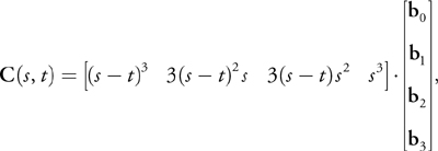
where the b i are cubic Bézier control points.
The first step is to compute the coefficients of the function I(s, t) whose roots correspond to inflection points of C(s, t). An inflection point is where the curve changes its bending direction, defined mathematically as parameter values where the first and second derivatives of C(s, t) are linearly dependent. The derivation of the function I is not needed for our current purposes; see Blinn 2003 for a thorough discussion. For integral cubic curves,
|
I(s, t) = t(3d 1 s 2 - 3d 2 st + d 3 t 2), |
where
|
d 1 = a 1 - 2a 2 + 3a 3, |
d 2 = -a 2 + 3a 3, |
d 3 = 3a 3 |
and
|
a 1 = b 0 · (b 3 x b 2), |
a 2 = b 1 · (b 0 x b 3), |
a 3 = b 2 · (b 1 x b 1). |
The function I is a cubic with three roots, not all necessarily real. It is the number of distinct real roots of I(s, t) that determines the type of the cubic curve. For integral cubic curves, [s t] = [1 0] is always a root of I(s, t). This means that the remaining roots of I(s, t) can be found using the quadratic formula, rather than by the more general solution of a cubic—a significant simplification over the general rational curve algorithm.
Our cubic curve classification reduces to knowing the sign of the discriminant of I(s, t), defined as
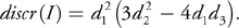
If discr(I) is positive, the curve is a serpentine; if negative, it is a loop; and if zero, a cusp. Although it is true that all cubic curves are one of these three types, not all configurations of four Bézier control points result in cubic curves. It is possible to represent quadratic curves, lines, or even single points in cubic Bézier form. Our procedure will detect these cases, and our rendering algorithm can handle them. We don't need to consider (or render) lines or points, because the convex hull of the Bézier control points in these cases has zero area and, therefore, no pixel coverage. The general classification of cubic Bézier curves is given by Table 25-1.
Table 25-1. Cubic Curve Classification
|
Serpentine |
discr(I) > 0 |
|
Cusp |
discr(I) = 0 |
|
Loop |
discr(I) < 0 |
|
Quadratic |
d 1 = d 2 = 0 |
|
Line |
d 1 = d 2 = d 3 = 0 |
|
Point |
b 0 = b 1 = b 2 = b 3 |
If our Bézier control points have exact floating-point coordinates, the classification given in Table 25-1 can be done exactly. That is, there is no ambiguity between cases, because discr(I) and all intermediate variables can be derived from exact floating representations.
Once a curve has been classified, we must find the texture coordinates [ki li mi ] corresponding to each Bézier control point b i , i = 0, 1, 2, 3. Our approach is to find scalarvalued cubic functions
|
k(s, t) = k . C(s, t), |
l(s, t), = l . C(s, t), |
m(s, t) = m . C(s, t), |
in Bézier form; the coefficients of these functions will correspond to our procedural texture coordinates. Because we know the geometry of the lines k, l, and m in Figure 25-4, we could find points and tangent vectors of C(s, t) and from these construct the needed lines. But lines are homogeneous, scale-invariant objects; what we need are the corresponding linear functionals, where (relative) scale matters.
Our strategy will be to construct k(s, t), l(s, t), and
m(s, t) by taking products of their linear factors. These linear factors are found by
solving for the roots of I(s, t) and a related polynomial called the Hessian
of I(s, t). For each curve type, we find the parameter values [ls
lt ] and [ms mt ] of I(s,
t) where k
l and k
m. We denote these linear factors by the following:
|
L
|
M
|
We can reason about how to construct k(s, t), l(s, t), and m(s, t) from L and M by studying the geometric relationship of C(s, t) to lines k, l, and m. For example, k(s, t) will have roots at [ls lt ], [ms mt ], and a root at infinity [1 0]. Therefore, for all cubic curves:
|
k(s, t) = LM. |
Finding the cubic functions l(s, t) and m(s, t) for each of the three curve types has its own reasoning, to be described shortly.
Once the functions k(s, t), l(s, t), and m(s, t) are known, we convert them to cubic Bézier form to obtain
where [ki li mi ] are the procedural texture coordinates associated with b i , i = 0, 1, 2, 3.
Finally, to make sure that the curve has the correct orientation—to the right is inside—we may need to reverse
orientation by multiplying the implicit equation by -1. This is equivalent to setting M
 M · O, where
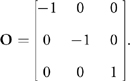
The conditions for correcting orientation depend on curve type, described next.
25.3.1 Serpentine
For a serpentine curve, C(s, t) is tangent to line l at the
inflection point where k
l. The scalar-valued function l(s, t) will also have an inflection
point at this parameter value; meaning that l(s, t) will have a triple root there. A
similar analysis applies for m(s, t). We form products of the linear factors to get
|
k(s, t) = LM, |
l(s, t) = L 3, |
m(s, t) = M 3. |
To find the parameter value of these linear factors, we compute the roots of I(s, t):
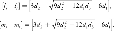
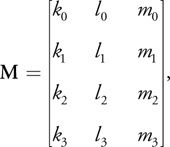
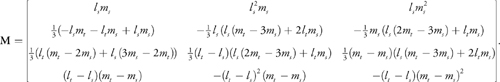
We convert k(s, t), l(s, t), and m(s, t) to cubic Bézier form and form the coefficient matrix
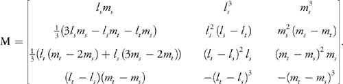
Each row of the M matrix corresponds to the procedural texture coordinate associated with the
Bézier curve control points. If d 1 < 0, then we must reverse orientation by setting
M
M · O.
25.3.2 Loop
For a loop curve, C(s, t) is tangent to line l and crosses line m at one of the double point parameters. This means that l(s, t) will have a double root at [ls lt ] and a single root at [ms mt ]. A similar analysis holds for m(s, t). We then take products of the linear factors to get
|
k(s, t) = LM, |
l(s, t) = L 2 M, |
m(s, t) = LM 2. |
The parameter values of the double point are found as roots of the Hessian of I(s, t), defined as
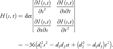
Because H(s, t) is quadratic, we use the quadratic formula to find the roots:
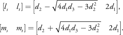
We convert k(s, t), l(s, t), and m(s, t) to cubic Bézier form to get
A rendering artifact will occur if one of the double point parameters lies in the interval [0/1, 1/1]. To solve
this problem, we subdivide the curve at the double point parameter—see
Figure 25-5—and reverse the orientation of one of the
subcurves. Note that the procedural texture coordinates of the subcurves can be found by subdividing the
procedural texture coordinates of the original curve. Once a loop curve has been sub divided at its double
point, the procedural texture coordinates ki , i = 0, . . ., 3 will have the same
sign. Orientation reversal (M
M · O) is needed if (d 1 > 0 and sign(k
1) < 0) or (d 1 < 0 and sign(k 1) > 0).
)
Figure 25-5 Cubic Curve with a Double Point
25.3.3 Cusp
A cusp occurs when discr(I) = 0. This is the boundary between the serpentine and loop cases. Geometrically, the lines l and m are coincident; therefore [ls lt ] = [ms mt ]. We could use the procedure for either the loop or the serpentine case, because the texture coordinate matrices will turn out to be the same.
There is an exception: when d 1 = 0. In the serpentine and loop cases, it must be that
d 1
 0; otherwise discr(I) = 0 and we would have a cusp. The case where d 1 = 0
and d 2
0
corresponds to a cubic curve that has a cusp at the parametric value [1 0]—that is, homogeneous infinity. In
this case, the inflection point polynomial reduces to
0; otherwise discr(I) = 0 and we would have a cusp. The case where d 1 = 0
and d 2
0
corresponds to a cubic curve that has a cusp at the parametric value [1 0]—that is, homogeneous infinity. In
this case, the inflection point polynomial reduces to
|
I(s, t) = t 2(d 3 t - 3d 2 s), |
which has a double root at infinity and a single root [ls lt ] = [d 3 3d 2]. We find
|
k(s, t) = L, |
l(s, t) = L 3, |
m(s, t) = 1. |
Converting these to Bézier form gives us the columns of the matrix:
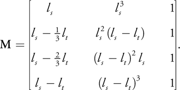
The orientation will never need to be reversed in this case. An example of a cubic curve whose inflection point polynomial has a cusp at infinity is [t t 3].
25.3.4 Quadratic
We showed earlier that quadratic curves could be rendered by a pixel shader that evaluated the expression
u 2 - v. Switching away from the cubic shader would be inefficient for the GPU, and
therefore undesirable. However, if we equate the cubic function k(s, t)
 m(s, t), our cubic shader expression can be written as
|
k 3 - kl = k(k 2 - l). |
We see that the part inside the parentheses is the quadratic shader expression with u and v replaced with k and l. The sign of this expression will agree with the quadratic shader, provided the value of k does not change sign inside the convex hull of the curve. We can degree-elevate the quadratic procedural texture coordinates to get
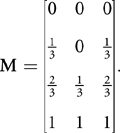
Interpolation will not change the sign of k in this case. Finally, we reverse orientation if d 3 < 0.
25.4 Triangulation
Our triangulation procedure was only briefly discussed in Sections 25.2 and 25.3 in the interest of simplicity. An important detail not previously mentioned is that Bézier convex hulls cannot overlap. There are two reasons for this: one is that overlapping triangles cause problems for triangulation code; the other is that unwanted portions of one filled region might show through to the other, resulting in a visual artifact. This problem can be resolved by subdividing one of the offending curves so that Bézier curve convex hulls no longer overlap, as shown in Figure 25-6.
)
Figure 25-6 Handling Overlapping Triangles
We locally triangulate all non-overlapping Bézier convex hulls. For quadratics, the Bézier convex hull is uniquely a triangle. For cubics, the Bézier convex hull may be a quad or a triangle. If it is a quad, we triangulate by choosing either diagonal. Next, the interior of the entire boundary is triangulated. The details of this procedure are beyond the scope of this chapter. Any triangulation procedure for a multicontour polygon will work.
Recently, Kokojima et al. 2006 presented a variant on our approach for quadratic splines that used the stencil buffer to avoid triangulation. Their idea is to connect all points on the curve path and draw them as a triangle fan into the stencil buffer with the invert operator. Only pixels drawn an odd number of times will be nonzero, thus giving the correct image of concavities and holes. Next, they draw the curve segments, treating them all as convex quadratic elements. This will either add to or carve away a curved portion of the shape. A quad large enough to cover the extent of the stencil buffer is then drawn to the frame buffer with a stencil test. The result is the same as ours without triangulation or subdivision, and needing only one quadratic curve orientation. Furthermore, eliminating the triangulation steps makes high-performance rendering of dynamic curves possible. The disadvantage of their approach is that two passes over the curve data are needed. For static curves, they are trading performance for implementation overhead.
25.5 Antialiasing
We present an approach to antialiasing in the pixel shader based on a signed distance approximation to a curve boundary. By reducing pixel opacity within a narrow band that contains the boundary, we can approximate convolution with a filter kernel. However, this works only when pixel samples lie on both sides of a boundary, such as points well inside the Bézier convex hull of a curve. For points near triangle edges, or when the edge of a triangle is the boundary, this scheme breaks down. Fortunately, this is exactly the case that is handled by hardware multisample antialiasing (MSAA). MSAA uses a coverage mask derived as the percentage of samples (from a hardware-dependent sample pattern) covered by a triangle. Only one pixel shader call is initiated, and this is optionally located at the centroid of the covered samples, as opposed to the pixel center, to avoid sampling outside the triangle's image in texture space. In our case, out-of-gamut sampling is not a problem, because we use a procedural definition of a texture (an algebraic equation). Therefore, centroid sampling is not recommended.
For antialiasing of curved boundaries on the interior of the Bézier convex hull, we need to know the screen-space signed distance from the current pixel to the boundary. If this distance is ±½ a pixel (an empirically determined choice; this could be less or more), then the opacity of the pixel color is changed relative to the pixel's distance to the curved boundary. Computing the true distance to a degree d polynomial curve requires the solution to a degree 2d - 1 equation. This is impractical on today's hardware, for performance reasons.
Instead, we use an approximate signed distance based on gradients. For a function f (x,
y), the gradient of f is a vector operator
 f
= [df/x f/y]. The GPU has hardware support for taking gradients of variables
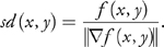
in pixel shader programs via the ddx() and ddy() functions. We define the signed distance
function to the screen-space curve f (x, y) = 0 to be
f
= [df/x f/y]. The GPU has hardware support for taking gradients of variables
in pixel shader programs via the ddx() and ddy() functions. We define the signed distance
function to the screen-space curve f (x, y) = 0 to be
In our case, the implicit function is not defined in screen (pixel) space. However, the process of interpolating procedural texture coordinates in screen space is, in effect, mapping screen [x y] space to procedural texture coordinate space ([u v] for quadratics, [k l m] for cubics). In other words, we can think of the interpolated procedural texture coordinates as vector functions
|
[u(x, y) |
v(x, y)] |
or |
[k(x, y) |
l(x, y) |
m(x, y)]. |
Each of these coordinate functions is actually the ratio of linear functionals whose quotient is taken in hardware (that is, perspective correction). An implicit function of these coordinate functions is a composition, defining a screen-space implicit function. Therefore, our signed distance function correctly measures approximate distance in pixel units.
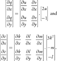
Hardware gradients are based on differences between values of adjacent pixels, so they can only approximate the derivatives of higher-order functions. Although this rarely (if ever) results in artifacts, with only a few additional math operations, we can get exact derivatives by applying the chain rule to our shader equations. Let the following,
|
q(x, y) = u(x, y)2 - v(x, y) = 0 and |
|
c(x, y) = k(x, y)3 - l(x, y)m(x, y) = 0, |
be our quadratic and cubic shader equations, respectively. Applying the chain rule, we get
We can write our signed distance function as
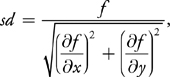
where f
q for quadratics and f
c for cubics. For a boundary interval of ±½ pixel, we map signed distance to opacity by a = ½
- sd. This is based on a linear ramp blending; higher-order blending could be used at higher cost. If
> 1, we set
1; if a < 0, we abort the pixel.
25.6 Code
Listing 25-1 is HLSL code for our quadratic shader. The code for the cubic shader is similar.
Example 25-1. Quadratic Curve Pixel Shader
float4 QuadraticPS(float2 p : TEXCOORD0, float4 color : COLOR0) : COLOR
{
  // Gradients
  float2 px = ddx(p);
  float2 py = ddy(p);
  // Chain rule
  float fx = (2 * p.x) * px.x - px.y;
  float fy = (2 * p.x) * py.x - py.y;
  // Signed distance
  float sd = (p.x * p.x - p.y) / sqrt(fx * fx + fy * fy);
  // Linear alpha
  float alpha = 0.5 - sd;
  if (alpha > 1)
    // Inside
    color.a = 1;
  else if (alpha < 0)
    // Outside
    clip(-1);
  else
    // Near boundary
    color.a = alpha;
  return color;
}
25.7 Conclusion
We have presented an algorithm for rendering vector art defined by closed paths containing quadratic and cubic Bézier curves. We locally triangulate each Bézier convex hull and globally triangulate the interior (right-hand side) of each path. We assign procedural texture coordinates to the vertices of each Bézier convex hull. These coordinates encode linear functionals and are interpolated by the hardware during rasterization. The process of interpolation maps the procedural texture coordinates to a space where the implicit equation of the curve has a simple form: u 2 - v = 0 for quadratics and k 3 - lm = 0 for cubics. A pixel shader program evaluates the implicit equation. The sign of the result will determine if a pixel is inside (negative) or outside (positive). We use hardware gradients to approximate a screen-space signed distance to the curve boundary. This signed distance is used for antialiasing the curved boundaries. We can apply an arbitrary projective transform to view our plane curves in 3D. The result has a small and static memory footprint, and the resulting image is resolution independent. Figure 25-7 shows an example of some text rendered in perspective using our technique.
)
Figure 25-7 Our Algorithm Is Used to Render 2D Text with Antialiasing Under a 3D Perspective Transform
In the future, we would like to extend this rendering paradigm to curves of degree 4 and higher. This would allow us to apply freeform deformations to low-order shapes (such as font glyphs) and have the resulting higher-order curve be resolution independent. The work of Kokojima et al. 2006 showed how to render dynamic quadratic curves; we would like to extend their approach to handle cubic curves as well. This is significantly more complicated than the quadratic case, because of the procedural texture-coordinate-assignment phase. However, it should be possible to do this entirely on the GPU using DirectX 10-class hardware equipped with a geometry shader (Blythe 2006).
25.8 References
Blinn, Jim. 2003. Jim Blinn's Corner: Notation, Notation, Notation. Morgan Kaufmann.
Blythe, David. 2006. "The Direct3D 10 System." In ACM Transactions on Graphics (Proceedings of SIGGRAPH 2006) 25(3), pp. 724–734.
Kokojima, Yoshiyuki, Kaoru Sugita, Takahiro Saito, and Takashi Takemoto. 2006. "Resolution Independent Rendering of Deformable Vector Objects using Graphics Hardware." In ACM SIGGRAPH 2006 Sketches.
Loop, Charles, and Jim Blinn. 2005. "Resolution Independent Curve Rendering using Programmable Graphics Hardware." In ACM Transactions on Graphics (Proceedings of SIGGRAPH 2005) 24(3), pp. 1000–1008.
Salmon, George. 1852. A Treatise on the Higher Order Plane Curves. Hodges & Smith.
- Contributors
- Foreword
- Part I: Geometry
-
- Chapter 1. Generating Complex Procedural Terrains Using the GPU
- Chapter 2. Animated Crowd Rendering
- Chapter 3. DirectX 10 Blend Shapes: Breaking the Limits
- Chapter 4. Next-Generation SpeedTree Rendering
- Chapter 5. Generic Adaptive Mesh Refinement
- Chapter 6. GPU-Generated Procedural Wind Animations for Trees
- Chapter 7. Point-Based Visualization of Metaballs on a GPU
- Part II: Light and Shadows
-
- Chapter 8. Summed-Area Variance Shadow Maps
- Chapter 9. Interactive Cinematic Relighting with Global Illumination
- Chapter 10. Parallel-Split Shadow Maps on Programmable GPUs
- Chapter 11. Efficient and Robust Shadow Volumes Using Hierarchical Occlusion Culling and Geometry Shaders
- Chapter 12. High-Quality Ambient Occlusion
- Chapter 13. Volumetric Light Scattering as a Post-Process
- Part III: Rendering
-
- Chapter 14. Advanced Techniques for Realistic Real-Time Skin Rendering
- Chapter 15. Playable Universal Capture
- Chapter 16. Vegetation Procedural Animation and Shading in Crysis
- Chapter 17. Robust Multiple Specular Reflections and Refractions
- Chapter 18. Relaxed Cone Stepping for Relief Mapping
- Chapter 19. Deferred Shading in Tabula Rasa
- Chapter 20. GPU-Based Importance Sampling
- Part IV: Image Effects
-
- Chapter 21. True Impostors
- Chapter 22. Baking Normal Maps on the GPU
- Chapter 23. High-Speed, Off-Screen Particles
- Chapter 24. The Importance of Being Linear
- Chapter 25. Rendering Vector Art on the GPU
- Chapter 26. Object Detection by Color: Using the GPU for Real-Time Video Image Processing
- Chapter 27. Motion Blur as a Post-Processing Effect
- Chapter 28. Practical Post-Process Depth of Field
- Part V: Physics Simulation
-
- Chapter 29. Real-Time Rigid Body Simulation on GPUs
- Chapter 30. Real-Time Simulation and Rendering of 3D Fluids
- Chapter 31. Fast N-Body Simulation with CUDA
- Chapter 32. Broad-Phase Collision Detection with CUDA
- Chapter 33. LCP Algorithms for Collision Detection Using CUDA
- Chapter 34. Signed Distance Fields Using Single-Pass GPU Scan Conversion of Tetrahedra
- Chapter 35. Fast Virus Signature Matching on the GPU
- Part VI: GPU Computing
-
- Chapter 36. AES Encryption and Decryption on the GPU
- Chapter 37. Efficient Random Number Generation and Application Using CUDA
- Chapter 38. Imaging Earth's Subsurface Using CUDA
- Chapter 39. Parallel Prefix Sum (Scan) with CUDA
- Chapter 40. Incremental Computation of the Gaussian
- Chapter 41. Using the Geometry Shader for Compact and Variable-Length GPU Feedback
- Preface