GPU Gems 3
GPU Gems 3 is now available for free online!
The CD content, including demos and content, is available on the web and for download.
You can also subscribe to our Developer News Feed to get notifications of new material on the site.
Chapter 18. Relaxed Cone Stepping for Relief Mapping
Fabio Policarpo
Perpetual Entertainment
Manuel M. Oliveira
Instituto de Informática—UFRGS
18.1 Introduction
The presence of geometric details on object surfaces dramatically changes the way light interacts with these surfaces. Although synthesizing realistic pictures requires simulating this interaction as faithfully as possible, explicitly modeling all the small details tends to be impractical. To address these issues, an image-based technique called relief mapping has recently been introduced for adding per-fragment details onto arbitrary polygonal models (Policarpo et al. 2005). The technique has been further extended to render correct silhouettes (Oliveira and Policarpo 2005) and to handle non-height-field surface details (Policarpo and Oliveira 2006). In all its variations, the ray-height-field intersection is performed using a binary search, which refines the result produced by some linear search procedure. While the binary search converges very fast, the linear search (required to avoid missing large structures) is prone to aliasing, by possibly missing some thin structures, as is evident in Figure 18-1a. Several space-leaping techniques have since been proposed to accelerate the ray-height-field intersection and to minimize the occurrence of aliasing (Donnelly 2005, Dummer 2006, Baboud and Décoret 2006). Cone step mapping (CSM) (Dummer 2006) provides a clever solution to accelerate the intersection calculation for the average case and avoids skipping height-field structures by using some precomputed data (a cone map). However, because CSM uses a conservative approach, the rays tend to stop before the actual surface, which introduces different kinds of artifacts, highlighted in Figure 18-1b. Using an extension to CSM that consists of employing four different radii for each fragment (in the directions north, south, east, and west), one can just slightly reduce the occurrence of these artifacts. We call this approach quad-directional cone step mapping (QDCSM). Its results are shown in Figure 18-1c, which also highlights the technique's artifacts.
)
Figure 18-1 Comparison of Four Different Ray-Height-Field Intersection Techniques Used to Render a Relief-Mapped Surface from a 256x256 Relief Texture
In this chapter, we describe a new ray-height-field intersection strategy for per-fragment displacement mapping that combines the strengths of both cone step mapping and binary search. We call the new space-leaping algorithm relaxed cone stepping (RCS), as it relaxes the restriction used to define the radii of the cones in CSM. The idea for the ray-height-field intersection is to replace the linear search with an aggressive spaceleaping approach, which is immediately followed by a binary search. While CSM conservatively defines the radii of the cones in such a way that a ray never pierces the surface, RCS allows the rays to pierce the surface at most once. This produces much wider cones, accelerating convergence. Once we know a ray is inside the surface, we can safely apply a binary search to refine the position of the intersection. The combination of RCS and binary search produces renderings of significantly higher quality, as shown in Figure 18-1d. Note that both the aliasing visible in Figure 18-1a and the distortions noticeable in Figures 18-1b and 18-1c have been removed. As a space-leaping technique, RCS can be used with other strategies for refining ray-height-field intersections, such as the one used by interval mapping (Risser et al. 2005).
18.2 A Brief Review of Relief Mapping
Relief mapping (Policarpo et al. 2005) simulates the appearance of geometric surface details by shading individual fragments in accordance to some depth and surface normal information that is mapped onto polygonal models. A depth map [1] (scaled to the [0,1] range) represents geometric details assumed to be under the polygonal surface. Depth and normal maps can be stored as a single RGBA texture (32-bit per texel) called a relief texture (Oliveira et al. 2000). For better results, we recommend separating the depth and normal components into two different textures. This way texture compression will work better, because a specialized normal compression can be used independent of the depth map compression, resulting in higher compression ratios and fewer artifacts. It also provides better performance because during the relief-mapping iterations, only the depth information is needed and a one-channel texture will be more cache friendly (the normal information will be needed only at the end for lighting). Figure 18-2 shows the normal and depth maps of a relief texture whose cross section is shown in Figure 18-3. The mapping of relief details to a polygonal model is done in the conventional way, by assigning a pair of texture coordinates to each vertex of the model. During rendering, the depth map can be dynamically rescaled to achieve different effects, and correct occlusion is achieved by properly updating the depth buffer.
)
Figure 18-2 Example of a Relief Texture
)
Figure 18-3 Relief Rendering
Relief rendering is performed entirely on the GPU and can be conceptually divided into three steps. For each fragment f with texture coordinates (s, t), first transform the view direction V to the tangent space of f. Then, find the intersection P of the transformed viewing ray against the depth map. Let (k, l) be the texture coordinates of such intersection point (see Figure 18-3). Finally, use the corresponding position of P, expressed in camera space, and the normal stored at (k, l) to shade f. Self-shadowing can be applied by checking whether the light ray reaches P before reaching any other point on the relief. Figure 18-3 illustrates the entire process. Proper occlusion among relief-mapped and other scene objects is achieved simply by updating the z-buffer with the z coordinate of P (expressed in camera space and after projection and division by w). This updated z-buffer also supports the combined use of shadow mapping (Williams 1978) with relief-mapped surfaces.
In practice, finding the intersection point P can be entirely performed in 2D texture space. Thus, let (u, v) be the 2D texture coordinates corresponding to the point where the viewing ray reaches depth = 1.0 (Figure 18-3). We compute (u, v) based on (s, t), on the transformed viewing direction and on the scaling factor applied to the depth map. We then perform the search for P by sampling the depth map, stepping from (s, t) to (u, v), and checking if the viewing ray has pierced the relief (that is, whether the depth along the viewing ray is bigger than the stored depth) before reaching (u, v). If we have found a place where the viewing ray is under the relief, the intersection P is refined using a binary search.
Although the binary search quickly converges to the intersection point and takes advantage of texture filtering, it could not be used in the beginning of the search process because it may miss some large structures. This situation is depicted in Figure 18-4a, where the depth value stored at the texture coordinates halfway from (s, t) and (u, v) is bigger than the depth value along the viewing ray at point 1, even though the ray has already pierced the surface. In this case, the binary search would incorrectly converge to point Q. To minimize such aliasing artifacts, Policarpo et al. (2005) used a linear search to restrict the binary search space. This is illustrated in Figure 18-4b, where the use of small steps leads to finding point 3 under the surface. Subsequently, points 2 and 3 are used as input to find the desired intersection using a binary search refinement. The linear search itself, however, is also prone to aliasing in the presence of thin structures, as can be seen in Figure 18-1a. This has motivated some researchers to propose the use of additional preprocessed data to avoid missing such thin structures (Donnelly 2005, Dummer 2006, Baboud and Décoret 2006). The technique described in this chapter was inspired by the cone step mapping work of Dummer, which is briefly described next.
)
Figure 18-4 Binary Versus Linear Search
18.3 Cone Step Mapping
Dummer's algorithm for computing the intersection between a ray and a height field avoids missing height-field details by using cone maps (Dummer 2006). A cone map associates a circular cone to each texel of the depth texture. The angle of each cone is the maximum angle that would not cause the cone to intersect the height field. This situation is illustrated in Figure 18-5 for the case of three texels at coordinates (s, t), (a, b), and (c, d), whose cones are shown in yellow, blue, and green, respectively.
)
Figure 18-5 Cone Step Mapping
Starting at fragment f, along the transformed viewing direction, the search for an intersection proceeds as follows: intersect the ray with the cone stored at (s, t), obtaining point 1 with texture coordinates (a, b). Then advance the ray by intersecting it with the cone stored at (a, b), thus obtaining point 2 at texture coordinates (c, d). Next, intersect the ray with the cone stored at (c, d), obtaining point 3, and so on. In the case of this simple example, point 3 coincides with the desired intersection. Although cone step mapping is guaranteed never to miss the first intersection of a ray with a height field, it may require too many steps to converge to the actual intersection. For performance reasons, however, one is often required to specify a maximum number of iterations. As a result, the ray tends to stop before the actual intersection, implying that the returned texture coordinates used to sample the normal and color maps are, in fact, incorrect. Moreover, the 3D position of the returned intersection, P', in camera space, is also incorrect. These errors present themselves as distortion artifacts in the rendered images, as can be seen in Figures 18-1b and 18-1c.
18.4 Relaxed Cone Stepping
Cone step mapping, as proposed by Dummer, replaces both the linear and binary search steps described in Policarpo et al. 2005 with a single search based on a cone map. A better and more efficient ray-height-field intersection algorithm is achieved by combining the strengths of both approaches: the space-leaping properties of cone step mapping followed by the better accuracy of the binary search. Because the binary search requires one input point to be under and another point to be over the relief surface, we can relax the constraint that the cones in a cone map cannot pierce the surface. In our new algorithm, instead, we force the cones to actually intersect the surface whenever possible. The idea is to make the radius of each cone as large as possible, observing the following constraint: As a viewing ray travels inside a cone, it cannot pierce the relief more than once. We call the resulting space-leaping algorithm relaxed cone stepping. Figure 18-7a (in the next subsection) compares the radii of the cones used by the conservative cone stepping (blue) and by relaxed cone stepping (green) for a given fragment in a height field. Note that the radius used by RCS is considerably larger, making the technique converge to the intersection using a smaller number of steps. The use of wider relaxed cones eliminates the need for the linear search and, consequently, its associated artifacts. As the ray pierces the surface once, it is safe to proceed with the fast and more accurate binary search.
18.4.1 Computing Relaxed Cone Maps
As in CSM, our approach requires that we assign a cone to each texel of the depth map. Each cone is represented by its width/height ratio (ratio w/h, in Figure 18-7c). Because a cone ratio can be stored in a single texture channel, both a depth and a cone map can be stored using a single luminance-alpha texture. Alternatively, the cone map could be stored in the blue channel of a relief texture (with the first two components of the normal stored in the red and green channels only).
For each reference texel ti on a relaxed cone map, the angle of cone Ci centered at ti is set so that no viewing ray can possibly hit the height field more than once while traveling inside Ci . Figure 18-7b illustrates this situation for a set of viewing rays and a given cone shown in green. Note that cone maps can also be used to accelerate the intersection of shadow rays with the height field. Figure 18-6 illustrates the rendering of self-shadowing, comparing the results obtained with three different approaches for rendering perfragment displacement mapping: (a) relief mapping using linear search, (b) cone step mapping, and (c) relief mapping using relaxed cone stepping. Note the shadow artifacts resulting from the linear search (a) and from the early stop of CSM (b).
)
Figure 18-6 Rendering Self-Shadowing Using Different Approaches
Relaxed cones allow rays to enter a relief surface but never leave it. We create relaxed cone maps offline using an O(n 2) algorithm described by the pseudocode shown in Listing 18-1. The idea is, for each source texel ti, trace a ray through each destination texel tj, such that this ray starts at (ti.texCoord.s, ti.texCoord.t, 0.0) and points to (tj.texCoord.s, tj.texCoord.t, tj.depth). For each such ray, compute its next (second) intersection with the height field and use this intersection point to compute the cone ratio cone_ratio(i,j). Figure 18-7c illustrates the situation for a given pair of (ti, tj) of source and destination texels. Ci 's final ratio is given by the smallest of all cone ratios computed for ti , which is shown in Figure 18-7b. The relaxed cone map is obtained after all texels have been processed as source texels.
)
Figure 18-7 Computing Relaxed Cone Maps
Example 18-1. Pseudocode for Computing Relaxed Cone Maps
 for each
   reference texel ti do radius_cone_C(i) = 1;
 source.xyz = (ti.texCoord.s, ti.texCoord.t, 0.0);
for each
  destination texel tj do destination.xyz =
      (tj.texCoord.s, tj.texCoord.t, tj.depth);
ray.origin = destination;
ray.direction = destination - source;
(k, w) = text_cords_next_intersection(tj, ray, depth_map);
d = depth_stored_at(k, w);
if ((d - ti.depth) > 0.0)
  // dst has to be above the src
  cone_ratio(i, j) = length(source.xy - destination.xy) / (d - tj.depth);
if (radius_cone_C(i) > cone_ratio(i, j))
  radius_cone_C(i) = cone_ratio(i, j);
Note that in the pseudocode shown in Listing 18-1, as well as in the actual code shown in Listing 18-2, we have clamped the maximum cone ratio values to 1.0. This is done to store the cone maps using integer textures. Although the use of floating-point textures would allow us to represent larger cone ratios with possible gains in space leaping, in practice we have observed that usually only a small subset of the texels in a cone map would be able to take advantage of that. This is illustrated in the relaxed cone map shown in Figure 18-8c. Only the saturated (white) texels would be candidates for having cone ratios bigger than 1.0.
)
Figure 18-8 A Comparison of Different Kinds of Cone Maps Computed for the Depth Map Shown in
Listing 18-2 presents a shader for generating relaxed cone maps. Figure 18-8 compares three different kinds of cone maps for the depth map associated with the relief texture shown in Figure 18-2. In Figure 18-8a, one sees a conventional cone map (Dummer 2006) stored using a single texture channel. In Figure 18-8b, we have a quad-directional cone map, which stores cone ratios for the four major directions into separate texture channels. Notice how different areas in the texture are assigned wider cones for different directions. Red texels indicate cones that are wider to the right, while green ones are wider to the left. Blue texels identify cones that are wider to the bottom, and black ones are wider to the top. Figure 18-8c shows the corresponding relaxed cone map, also stored using a single texture channel. Note that its texels are much brighter than the corresponding ones in the conventional cone map in Figure 18-8a, revealing its wider cones.
Example 18-2. A Preprocess Shader for Generating Relaxed Cone Maps
float4 depth2relaxedcone(in float2 TexCoord
                         : TEXCOORD0, in Sampler2D ReliefSampler,
                           in float3 Offset)
    : COLOR
{
  const int search_steps = 128;
  float3 src = float3(TexCoord, 0);
  // Source texel
  float3 dst = src + Offset;
  // Destination texel
  dst.z = tex2D(ReliefSampler, dst.xy).w;
  // Set dest. depth
  float3 vec = dst - src; // Ray direction
  vec /= vec.z;
  // Scale ray direction so that vec.z = 1.0
  vec *= 1.0 - dst.z;
  // Scale again
  float3 step_fwd = vec / search_steps;
  // Length of a forward step
  // Search until a new point outside the surface
  float3 ray_pos = dst + step_fwd;
  for (int i = 1; i < search_steps; i++)
  {
    float current_depth = tex2D(ReliefSampler, ray_pos.xy).w;
    if (current_depth < = ray_pos.z)
      ray_pos += step_fwd;
  }
  // Original texel depth
  float src_texel_depth = tex2D(ReliefSampler, TexCoord).w;
  // Compute the cone ratio
  float cone_ratio =
      (ray_pos.z > = src_texel_depth)
          ? 1.0
          : length(ray_pos.xy - TexCoord) / (src_texel_depth - ray_pos.z);
  // Check for minimum value with previous pass result
  float best_ratio = tex2D(ResultSampler, TexCoord).x;
  if (cone_ratio > best_ratio)
    cone_ratio = best_ratio;
  return float4(cone_ratio, cone_ratio, cone_ratio, cone_ratio);
}
18.4.2 Rendering with Relaxed Cone Maps
To shade a fragment, we step along the viewing ray as it travels through the depth texture, using the relaxed cone map for space leaping. We proceed along the ray until we reach a point inside the relief surface. The process is similar to what we described in Section 18.3 for conventional cone maps. Figure 18-9 illustrates how to find the intersection between a transformed viewing ray and a cone. First, we scale the vector representing the ray direction by dividing it by its z component (ray.direction.z), after which, according to Figure 18-9, one can write
Equation 1
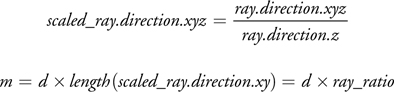
Likewise:
Equation 2
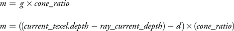
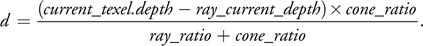
Solving Equations 1 and 2 for d gives the following:
Equation 3
From Equation 3, we compute the intersection point I as this:
Equation 4

)
Figure 18-9 Intersecting the Viewing Ray with a Cone
The code in Listing 18-3 shows the ray-intersection function for relaxed cone stepping. For performance reasons, the first loop iterates through the relaxed cones for a fixed number of steps. Note the use of the saturate() function when calculating the distance to move. This guarantees that we stop on the first visited texel for which the viewing ray is under the relief surface. At the end of this process, we assume the ray has pierced the surface once and then start the binary search for refining the coordinates of the intersection point. Given such coordinates, we then shade the fragment as described in Section 18.2.
Example 18-3. Ray Intersect with Relaxed Cone
// Ray intersect depth map using relaxed cone stepping.
// Depth value stored in alpha channel (black at object surface)
// and relaxed cone ratio stored in blue channel.
void ray_intersect_relaxedcone(sampler2D relief_map,
                               // Relaxed cone map
                               inout float3 ray_pos,
                               // Ray position
                               inout float3 ray_dir)
// Ray direction
{
  const int cone_steps = 15;
  const int binary_steps = 6;
  ray_dir /= ray_dir.z;
  // Scale ray_dir
  float ray_ratio = length(ray_dir.xy);
  float3 pos = ray_pos;
  for (int i = 0; i < cone_steps; i++)
  {
    float4 tex = tex2D(relief_map, pos.xy);
    float cone_ratio = tex.z;
    float height = saturate(tex.w – pos.z);
    float d = cone_ratio * height / (ray_ratio + cone_ratio);
    pos += ray_dir * d;
  }
  // Binary search initial range and initial position
  float3 bs_range = 0.5 * ray_dir * pos.z;
  float3 bs_position = ray_pos + bs_range;
  for (int i = 0; i < binary_steps; i++)
  {
    float4 tex = tex2D(relief_map, bs_position.xy);
    bs_range *= 0.5;
    if (bs_position.z < tex.w)
      // If outside
      bs_position += bs_range;
    // Move forward
    else
      bs_position -= bs_range;
    // Move backward
  }
}
Let f be the fragment to be shaded and let K be the point where the viewing ray has stopped (that is, just before performing the binary search), as illustrated in Figure 18-10. If too few steps were used, the ray may have stopped before reaching the surface. Thus, to avoid skipping even thin height-field structures (see the example shown in Figure 18-4a), we use K as the end point for the binary search. In this case, if the ray has not pierced the surface, the search will converge to point K.
)
Figure 18-10 The Viewing Ray Through Fragment , with Texture Coordinates ()
Let (m, n) be the texture coordinates associated to K and let dK be the depth value stored at (m, n) (see Figure 18-10). The binary search will then look for an intersection along the line segment ranging from points H to K, which corresponds to texture coordinates ((s + m)/2, (t+n)/2) to (m, n), where (s, t) are the texture coordinates of fragment f (Figure 18-10). Along this segment, the depth of the viewing ray varies linearly from (dK /2) to dK . Note that, instead, one could use (m, n) and (q, r) (the texture coordinates of point J, the previously visited point along the ray) as the limits for starting the binary search refinement. However, because we are using a fixed number of iterations for stepping over the relaxed cone map, saving (q, r) would require a conditional statement in the code. According to our experience, this tends to increase the number of registers used in the fragment shader. The graphics hardware has a fixed number of registers and it runs as many threads as it can fit in its register pool. The fewer registers we use, the more threads we will have running at the same time. The latency imposed by the large number of dependent texture reads in relief mapping is hidden when multiple threads are running simultaneously. More-complex code in the loops will increase the number of registers used and thus reduce the number of parallel threads, exposing the latency from the dependent texture reads and reducing the frame rate considerably. So, to keep the shader code shorter, we start the binary search using H and K as limits. Note that after only two iterations of the binary search, one can expect to have reached a search range no bigger than the one defined by the points J and K.
It should be clear that the use of relaxed cone maps could still potentially lead to some distortion artifacts similar to the ones produced by regular (conservative) cone maps (Figure 18-1b). In practice, they tend to be significantly less pronounced for the same number of steps, due to the use of wider cones. According to our experience, the use of 15 relaxed cone steps seems to be sufficient to avoid such artifacts in typical height fields.
18.5 Conclusion
The combined use of relaxed cone stepping and binary search for computing rayheight-field intersection significantly reduces the occurrence of artifacts in images generated with per-fragment displacement mapping. The wider cones lead to more-efficient space leaping, whereas the binary search accounts for more accuracy. If too few cone stepping iterations are used, the final image might present artifacts similar to the ones found in cone step mapping (Dummer 2006). In practice, however, our technique tends to produce significantly better results for the same number of iterations or texture accesses. This is an advantage, especially for the new generations of GPUs, because although both texture sampling and computation performance have been consistently improved, computation performance is scaling faster than bandwidth.
Relaxed cone stepping integrates itself with relief mapping in a very natural way, preserving all of its original features. Figure 18-11 illustrates the use of RCS in renderings involving depth scaling (Figures 18-11b and 18-11d) and changes in tiling factors (Figures 18-11c and 18-11d). Note that these effects are obtained by appropriately adjusting the directions of the viewing rays (Policarpo et al. 2005) and, therefore, not affecting the cone ratios.
)
Figure 18-11 Images Showing Changes in Apparent Depth and Tiling Factors
Mipmapping can be safely applied to color and normal maps. Unfortunately, conventional mipmapping should not be applied to cone maps, because the filtered values would lead to incorrect intersections. Instead, one should compute the mipmaps manually, by conservatively taking the minimum value for each group of pixels. Alternatively, one can sample the cone maps using a nearest-neighbors strategy. In this case, when an object is seen from a distance, the properly sampled color texture tends to hide the aliasing artifacts resulting from the sampling of a high-resolution cone map. Thus, in practice, the only drawback of not applying mipmapping to the cone map is the performance penalty for not taking advantage of sampling smaller textures.
18.5.1 Further Reading
Relief texture mapping was introduced in Oliveira et al. 2000 using a two-pass approach consisting of a prewarp followed by conventional texture mapping. The prewarp, based on the depth map, was implemented on the CPU and the resulting texture sent to the graphics hardware for the final mapping. With the introduction of fragment processors, Policarpo et al. (2005) generalized the technique for arbitrary polygonal models and showed how to efficiently implement it on a GPU. This was achieved by performing the ray-height-field intersection in 2D texture space. Oliveira and Policarpo (2005) also described how to render curved silhouettes by fitting a quadric surface at each vertex of the model. Later, they showed how to render relief details in preexisting applications using a minimally invasive approach (Policarpo and Oliveira 2006a). They have also generalized the technique to map non-height-field structures onto polygonal models and introduced a new class of impostors (Policarpo and Oliveira 2006b). More recently, Oliveira and Brauwers (2007) have shown how to use a 2D texture approach to intersect rays against depth maps generated under perspective projection and how to use these results to render real-time refractions of distant environments through deforming objects.
18.6 References
Baboud, Lionel, and Xavier Décoret. 2006. "Rendering Geometry with Relief Textures." In Proceedings of Graphics Interface 2006.
Donnelly, William. 2005. "Per-Pixel Displacement Mapping with Distance Functions." In GPU Gems 2, edited by Matt Pharr, pp. 123–136. Addison-Wesley.
Dummer, Jonathan. 2006. "Cone Step Mapping: An Iterative Ray-Heightfield Intersection Algorithm." Available online at http://www.lonesock.net/files/ConeStepMapping.pdf.
Oliveira, Manuel M., Gary Bishop, and David McAllister. 2000. "Relief Texture Mapping." In Proceedings of SIGGRAPH 2000, pp. 359–368.
Oliveira, Manuel M., and Fabio Policarpo. 2005. "An Efficient Representation for Surface Details." UFRGS Technical Report RP-351. Available online at http://www.inf.ufrgs.br/~oliveira/pubs_files/Oliveira_Policarpo_RP-351_Jan_2005.pdf.
Oliveira, Manuel M., and Maicon Brauwers. 2007. "Real-Time Refraction Through Deformable Objects." In Proceedings of the 2007 Symposium on Interactive 3D Graphics and Games, pp. 89–96.
Policarpo, Fabio, Manuel M. Oliveira, and João Comba. 2005. "Real-Time Relief Mapping on Arbitrary Polygonal Surfaces." In Proceedings of the 2005 Symposium on Interactive 3D Graphics and Games, pp. 155–162.
Policarpo, Fabio, and Manuel M. Oliveira. 2006a. "Rendering Surface Details in Games with Relief Mapping Using a Minimally Invasive Approach." In SHADER X4: Advance Rendering Techniques, edited by Wolfgang Engel, pp. 109–119. Charles River Media, Inc.
Policarpo, Fabio, and Manuel M. Oliveira. 2006b. "Relief Mapping of Non-Height-Field Surface Details." In Proceedings of the 2006 Symposium on Interactive 3D Graphics and Games, pp. 55–62.
Risser, Eric, Musawir Shah, and Sumanta Pattanaik. 2005. "Interval Mapping." University of Central Florida Technical Report. Available online at http://graphics.cs.ucf.edu/IntervalMapping/images/IntervalMapping.pdf.
Williams, Lance. 1978. "Casting Curved Shadows on Curved Surfaces." In Computer Graphics (Proceedings of SIGGRAPH 1978) 12(3), pp. 270–274.
- Contributors
- Foreword
- Part I: Geometry
-
- Chapter 1. Generating Complex Procedural Terrains Using the GPU
- Chapter 2. Animated Crowd Rendering
- Chapter 3. DirectX 10 Blend Shapes: Breaking the Limits
- Chapter 4. Next-Generation SpeedTree Rendering
- Chapter 5. Generic Adaptive Mesh Refinement
- Chapter 6. GPU-Generated Procedural Wind Animations for Trees
- Chapter 7. Point-Based Visualization of Metaballs on a GPU
- Part II: Light and Shadows
-
- Chapter 8. Summed-Area Variance Shadow Maps
- Chapter 9. Interactive Cinematic Relighting with Global Illumination
- Chapter 10. Parallel-Split Shadow Maps on Programmable GPUs
- Chapter 11. Efficient and Robust Shadow Volumes Using Hierarchical Occlusion Culling and Geometry Shaders
- Chapter 12. High-Quality Ambient Occlusion
- Chapter 13. Volumetric Light Scattering as a Post-Process
- Part III: Rendering
-
- Chapter 14. Advanced Techniques for Realistic Real-Time Skin Rendering
- Chapter 15. Playable Universal Capture
- Chapter 16. Vegetation Procedural Animation and Shading in Crysis
- Chapter 17. Robust Multiple Specular Reflections and Refractions
- Chapter 18. Relaxed Cone Stepping for Relief Mapping
- Chapter 19. Deferred Shading in Tabula Rasa
- Chapter 20. GPU-Based Importance Sampling
- Part IV: Image Effects
-
- Chapter 21. True Impostors
- Chapter 22. Baking Normal Maps on the GPU
- Chapter 23. High-Speed, Off-Screen Particles
- Chapter 24. The Importance of Being Linear
- Chapter 25. Rendering Vector Art on the GPU
- Chapter 26. Object Detection by Color: Using the GPU for Real-Time Video Image Processing
- Chapter 27. Motion Blur as a Post-Processing Effect
- Chapter 28. Practical Post-Process Depth of Field
- Part V: Physics Simulation
-
- Chapter 29. Real-Time Rigid Body Simulation on GPUs
- Chapter 30. Real-Time Simulation and Rendering of 3D Fluids
- Chapter 31. Fast N-Body Simulation with CUDA
- Chapter 32. Broad-Phase Collision Detection with CUDA
- Chapter 33. LCP Algorithms for Collision Detection Using CUDA
- Chapter 34. Signed Distance Fields Using Single-Pass GPU Scan Conversion of Tetrahedra
- Chapter 35. Fast Virus Signature Matching on the GPU
- Part VI: GPU Computing
-
- Chapter 36. AES Encryption and Decryption on the GPU
- Chapter 37. Efficient Random Number Generation and Application Using CUDA
- Chapter 38. Imaging Earth's Subsurface Using CUDA
- Chapter 39. Parallel Prefix Sum (Scan) with CUDA
- Chapter 40. Incremental Computation of the Gaussian
- Chapter 41. Using the Geometry Shader for Compact and Variable-Length GPU Feedback
- Preface