GPU Gems 3

GPU Gems 3 is now available for free online!

The CD content, including demos and content, is available on the web and for download.

You can also subscribe to our Developer News Feed to get notifications of new material on the site.

Chapter 17. Robust Multiple Specular Reflections and Refractions

Tamás Umenhoffer
Budapest University of Technology and Economics

Gustavo Patow
University of Girona

László Szirmay-Kalos
Budapest University of Technology and Economics

In this chapter, we present a robust algorithm to compute single and multiple reflections and refractions on the GPU. To allow the fragment shader to access the geometric description of the whole scene when looking for the hit points of secondary rays, we first render the scene into a layered distance map. Each layer is stored as a cube map in the texture memory. The texels of these cube maps contain not only color information, but also the distance from a reference point and the surface normal, so the texels can be interpreted as sampled representations of the scene. The algorithm searches this representation to trace secondary rays. The search process starts with ray marching, which makes sure that no ray surface intersection is missed, and continues with a secant search, which provides accuracy.

After we introduce the general machinery for tracing secondary rays, we present the applications, including single and multiple reflections and refractions on curved surfaces. To compute multiple reflections and refractions, the normal vector stored at the distance maps is read and used to generate the reflected/refracted rays. These higher-order rays are traced similar to how the first reflection ray was traced by the fragment shader. The intensity of the reflected ray is calculated according to a simplified Fresnel formula that is also appropriate for metals. The resulting algorithm is simple to implement, runs in real time, and is accurate enough to render self-reflections. The implementation of our proposed method requires dynamic branching support.

17.1 Introduction

Image synthesis computes the radiance of points that are visible through the pixels of the virtual camera. Local illumination models compute the radiance from local properties—such as the position, normal vector, and material data—in addition to global light source parameters. Each point is shaded independently, which opens up a lot of possibilities for parallel computation. This independent and parallel shading concept is heavily exploited in current GPUs, owing its appealing performance to the parallel architecture made possible by the local illumination model. However, for ideal reflectors and refractors, the radiance of a point depends also on the illumination of other points; thus, points cannot be shaded independently. This condition means that the radiance computation of a point recursively generates new visibility and color computation tasks to determine the intensity of the indirect illumination.

The basic operation for solving the visibility problem of a point at a direction is to trace a ray. To obtain a complete path, we should continue ray tracing at the hit point to get a second point and further scattering points. GPUs trace rays of the same origin very efficiently, taking a "photo" from the shared ray origin and using the fragment shader unit to compute the radiance of the visible points. The photographic process involves rasterizing the scene geometry and exploiting the z-buffer to find the first hits of the rays passing through the pixels.

This approach is ideal for primary rays, but not for the secondary rays needed for the specular reflection and refraction terms of the radiance, because these rays do not share the same origin. To trace these rays, the fragment shader should have access to the scene. Because fragment shaders may access global (that is, uniform) parameters and textures, this requirement can be met if the scene geometry is stored in uniform parameters or in textures.

Scene objects can be encoded as the set of parameters of the surface equation, similar to classical ray tracing (Havran 2001, Purcell et al. 2002, and Purcell et al. 2003). If the scene geometry is too complex, simple proxy geometries can be used that allow fast approximate intersections (Bjorke 2004 and Popescu et al. 2006).

On the other hand, the scene geometry can also be stored in a sampled form. The oldest application of this idea is the depth map used by shadow algorithms (Williams 1978), which stores light-space z coordinates for the part of the geometry that is seen from the light position through a window.

To consider all directions, we should use a cube map instead of a single depth image. If we store world-space Euclidean distance in texels, the cube map becomes similar to a sphere map (Patow 1995 and Szirmay-Kalos et al. 2005). Thus, a pair of direction and distance values specifies the point visible at this direction, without knowing the orientation of the cube-map faces. This property is particularly important when we interpolate between two directions, because it relieves us from taking care of cube-map face boundaries. These cube maps that store distance values are called distance maps.

A depth or distance cube map represents only the surfaces directly visible from the eye position that was used to generate this map. The used eye position is called the reference point of the map. To also include surfaces that are occluded from the reference point, we should generate and store several layers of the distance map (in a texel we store not only the closest point, but all points that are in this direction).

In this chapter, we present a simple and robust ray-tracing algorithm that computes intersections with the geometry stored in layered distance maps. Note that this map is the sampled representation of the scene geometry. Thus, when a ray is traced, the intersection calculation can use this information instead of the triangular meshes. Fragment shaders can look up texture maps but cannot directly access meshes, so this replacement is crucial for the GPU implementation. In our approach, ray tracing may support searches for the second and third (and so on) hit points of the path, while the first point is identified by rasterization. Our approach can be considered an extension to environment mapping because it puts distance information into texels in order to obtain more-accurate ray environment intersections.

This robust machinery for tracing secondary rays can be used to compute real-time, multiple reflections and refractions.

17.2 Tracing Secondary Rays

The proposed ray tracing algorithm works on geometry stored in layered distance maps. A single layer of these layered distance maps is a cube map, where a texel contains the material properties, the distance, and the normal vector of the point that is in the direction of the texel. The material property is the reflected radiance for diffuse surfaces and the Fresnel factor at perpendicular illumination for specular reflectors. For refractors, the index of refraction is also stored as a material property. The distance is measured from the center of the cube map (that is, from the reference point).

17.2.1 Generation of Layered Distance Maps

Computing distance maps is similar to computing classical environment maps. We render the scene six times, taking the reference point as the eye and the faces of a cube as the window rectangles. The difference is that not only is the color calculated and stored in additional cube maps, but also the distance and the normal vector. We can generate the texture storing the color, plus the texture encoding the normal vector and the distance, in a single rendering pass, using the multiple render target feature.

The set of layers representing the scene could be obtained by depth peeling (Everitt 2001 and Liu et al. 2006) in the general case. To control the number of layers, we can limit the number of peeling passes, so we put far objects into a single layer whether or not they occlude each other, as shown in Figure 17-1. If the distance of far objects is significantly larger than the size of the reflective object, this approximation is acceptable.

Figure 17-1 A Layered Distance Map with 3 + 1 Layers

For simpler reflective objects that are not too close to the environment, the layer generation can be further simplified. The reference point is put at the center of the reflective object, and the front and back faces of the reflective object are rendered separately into two layers. Note that this method may not fill all texels of a layer, so some texels may represent no visible point. If we clear the render target with a negative distance value before rendering, then invalid texels containing no visible point can be recognized later by checking the sign of the distance.

When scene objects are moving, distance maps should be updated.

17.2.2 Ray Tracing Layered Distance Maps

The basic idea is discussed using the notations of Figure 17-2. The place vectors of points are represented by lowercase letters and the direction vectors are indicated by uppercase letters. Let us assume that center o of our coordinate system is the reference point and that we are interested in the illumination of point x from direction R.

Figure 17-2 Tracing a Ray from at Direction

The illuminating point is thus on the ray of equation x + R · d, where d is the parameter of the ray that needs to be determined. We can check the accuracy of an arbitrary approximation of d by reading the distance of the environment surface stored with the direction of l = x + R · d in the cube map (|l'|) and comparing it with the distance of approximating point l on the ray |l|. If |l| |l'|, then we have found the intersection. If the point on the ray is in front of the surface, that is |l| < |l'|, the current approximation is undershooting. On the other hand, when point |l| is behind the surface (|l| > |l'|), the approximation is overshooting.

Ray parameter d can be found by using an iterative process. The process starts with ray marching (that is, a linear search) and continues with a secant search. The robust linear search computes a rough overshooting guess and an undershooting approximation that enclose the first intersection of the ray. Starting with these approximations, the secant search quickly obtains an accurate intersection.

Linear Search

The possible intersection points are on the ray. Thus, the intersection can be found by marching on the ray (that is, checking points r(d) = x + R · d generated with an increasing sequence of positive parameter d, and detecting the first pair of subsequent points where one point is overshooting while the other is undershooting). The real intersection, then, lies between these two guesses and is found by using a secant search (discussed in the following subsection).

The definition of the increments of ray parameter d needs special consideration because now the geometry is sampled, and it is not worth checking the same sample many times while ignoring other samples. Unfortunately, making uniform steps on the ray does not guarantee that the texture space is uniformly sampled. As we get farther from the reference point, unit-length steps on the ray correspond to smaller steps in texture space. This problem can be solved by marching on a line segment that looks identical to the ray from the reference point, except that its two end points are at the same distance. The end points of such a line segment can be obtained by projecting the start of the ray, r(0) and the end of the ray, r() onto a unit sphere, resulting in new start s = x/|x| and end point e = R/|R|, respectively. The intersection must be found at the texels that are seen at a direction between s and e, as shown in Figure 17-3.

Figure 17-3 Marching on the Ray, Making Uniform Steps in Texture Space

The intersection algorithm searches these texels, making uniform steps on the line segment of s and e:

r'(t) = s · (1 - t) + e · t,

t = 0,t, 2t,..., 1.

The correspondence between ray parameter d and parameter t can be found by projecting r' onto the ray, which leads to the following formula:

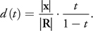
A fragment shader implementation should take inputs of the ray of origin x and direction R—as well as cube map map of type samplerCUBE passed as a uniform parameter—and sequentially generate ray parameters d and points on the ray r, and return an undershooting ray parameter dl and an overshooting ray parameter dp. Ratios |l|/|l'| and |p| / |p'| are represented by variables llp and ppp, respectively. The distance values are stored in the alpha channel of the cube map. Listing 17-1 shows the algorithm for the fragment shader executing a linear search.

This algorithm finds a pair of subsequent undershooting and overshooting points in a single layer, advancing on the ray making uniform steps Dt in texture space. Step size Dt is set proportionally to the length of line segment of s and e and to the resolution of the cube map. By setting texel step Dt to be greater than the distance of two neighboring texels, we speed up the algorithm but also increase the probability of missing the reflection of a thin object. At a texel, the distance value is obtained from the alpha channel of the cube map. Note that we use function texCUBElod()—setting the mipmap level explicitly to 0—instead of texCUBE(), because texCUBE(), like tex2D(), would force the DirectX 9 HLSL compiler to unroll the dynamic loop (Sander 2005).

Linear search should be run for each layer. The layer where the ray parameter (dp) is minimal contains the first hit of the ray.

Acceleration with Min-Max Distance Values

To speed up the intersection search in a layer, we compute a minimum and a maximum distance value for each distance map. When a ray is traced, the ray is intersected with the spheres centered at the reference point and having radii equal to the minimum and maximum values. The two intersection points significantly reduce the ray space that needs to be marched. This process moves the start point s and end point e closer, so fewer marching steps would provide the same accuracy. See Figure 17-4.

Figure 17-4 Min-Max Acceleration

Example 17-1. The Fragment Shader Executing a Linear Search in HLSL

    float a = length(x) / length(R); bool undershoot = false, overshoot = false; float dl, llp;  // Ray parameter and |l|/|l'| of last undershooting    float dp, ppp;  // Ray parameter and |p|/|p'| of last overshooting    float t = 0.0001f; while( t < 1 && !(overshoot && undershoot) ) {  // Iteration    float d = a * t / (1-t);  // Ray parameter corresponding to t    float3 r = x + R * d;  // r(d): point on the ray    float ra = texCUBElod(map, float4(r,0)).a; // |r'|    if (ra > 0) {  // Valid texel, i.e. anything is visible    float rrp = length(r)/ra; //|r|/|r'|    if (rrp < 1) {  // Undershooting       dl = d;  // Store last undershooting in dl       llp = rrp;       undershoot = true;     } else {  // Overshooting       dp = d;   // Store last overshooting as dp       ppp = rrp;       overshoot = true;     }   } else {  // Nothing is visible: restart search     undershoot = false;     overshoot = false;  }  t += Dt;  // Next texel }

Refinement by Secant Search

A linear search provides the first undershooting and overshooting pair of subsequent samples, so the real intersection must lie between these points. Let us denote the undershooting and overshooting ray parameters by d_p and d_l , respectively. The corresponding two points on the ray are p and l and the two points on the surface are p' and l', respectively, as shown in Figure 17-5.

Figure 17-5 Refinement by a Secant Step

Assuming that the surface is planar between points p' and l', we observe that it is intersected by the ray at point r = x + R · d_new , where

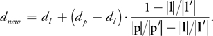
If a single secant step does not provide accurate enough results, then d_new can replace one of the previous approximations d_l or d_p (always keeping one overshooting and one undershooting approximation) and we can proceed with the same iteration step. Note that a secant search obtains exact results for planar surfaces in a single iteration step and requires just finite steps for planar meshes. Listing 17-2 shows the fragment shader implementation of the secant search.

Example 17-2. The Fragment Shader Implementation of the Secant Search in HLSL

    for(int i = 0; i < NITER; i++) {   // Ray parameter of the new intersection   dnew = dl + (dp-dl) * (1-llp)/(ppp-llp);   float3 r = x + R * dnew;  // New point on the ray    float rrp = length(r)/ texCUBElod(map, float4(r,0)).a; // |r|/|r'|    if (rrp < 0.9999) {  // Undershooting     llp = rrp;  // Store as last undershooting     dl = dnew;   } else if (rrp > 1.0001) {  // Overshooting     ppp = rrp;  // Store as last overshooting     dp = dnew;   } else i = NITER; }

We put the linear search executed for every layer, plus the secant search that processes a single layer, together in a Hit() function. We now have a general tool to trace an arbitrary ray in the scene. This function finds the first hit l. Reading the cube maps in this direction, we can obtain the material properties and the normal vector associated with this point.

17.3 Reflections and Refractions

Let us first consider specular reflections. Having generated the layered distance map, we render the reflective objects and activate custom vertex and fragment shader programs. The vertex shader transforms the reflective object to clipping space—and also to the coordinate system of the cube map—by first applying the modeling transform, then translating to the reference point. View vector V and normal N are also obtained in this space. Listing 17-3 shows the vertex shader of reflections and refractions.

Example 17-3. The Vertex Shader of Reflections and Refractions in HLSL

    void SpecularReflectionVS(    in float4 Pos  : POSITION,   // Vertex in modeling space    in float3 Norm : NORMAL,     // Normal in modeling space    out float4 hPos : POSITION,   // Vertex in clip space    out float3 x    : TEXCOORD1,  // Vertex in cube-map space    out float3 N    : TEXCOORD2,  // Normal in cube-map space    out float3 V    : TEXCOORD3,  // View direction    uniform float4x4 WorldViewProj,  // Modeling to clip space    uniform float4x4 World,          // Modeling to world space    uniform float4x4 WorldIT,        // Inverse-transpose of World    uniform float3   RefPoint,       // Reference point in world space    uniform float3   EyePos          // Eye in world space ) {   hPos = mul(Pos, WorldViewProj);   float3 wPos = mul(Pos, World).xyz;  // World space   N = mul(Norm, WorldIT);   V = wPos - EyePos;   x = wPos - RefPoint;  // Translate to cube-map space }

The fragment shader calls the function Hit() that returns the first hit l, its radiance Il, and normal vector Nl. If the surface is an ideal mirror, the incoming radiance should be multiplied by the Fresnel term evaluated for the angle between surface normal N and reflection direction R. We apply an approximation of the Fresnel function (Schlick 1993), which takes into account not only refraction index n, but also extinction coefficient k (which is essential for realistic metals) (Bjorke 2004; Lazányi and Szirmay-Kalos 2005):

F(N,R) = F_p + (1 - F _p )·(1 - N · R)⁵,

where

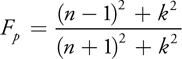
is the Fresnel function (that is, the probability that the photon is reflected) at perpendicular illumination. Note that F_p is constant for a given material. Thus, this value can be computed on the CPU from the refraction index and the extinction coefficient and passed to the GPU as a global variable. Listing 17-4 shows the fragment shader of single reflection.

Example 17-4. The Fragment Shader of Single Reflection in HLSL

    float4 SingleReflectionPS(   float3 x : TEXCOORD1,  // Shaded point in cube-map space    float3 N : TEXCOORD2,  // Normal vector    float3 V : TEXCOORD3,  // View direction    uniform float3 Fp0  // Fresnel at perpendicular direction ) : COLOR {   V = normalize(V);   N = normalize(N);   float3 R = reflect(V, N); // Reflection direction    float3 Nl;  // Normal vector at the hit point    float3 Il;  // Radiance at the hit point    // Trace ray x+R*d and obtain hit l, radiance Il, normal Nl    float3 l = Hit(x, R, Il, Nl);   // Fresnel reflection    float3 F = Fp0 + pow(1-dot(N, -V), 5) * (1-Fp0);   return float4(F * Il, 1); }

The shader of single refraction is similar, but the direction computation should use the law of refraction instead of the law of reflection. In other words, the reflect operation should be replaced by the refract operation, and the incoming radiance should be multiplied by 1-F instead of F.

Light may get reflected or refracted on ideal reflectors or refractors several times before it arrives at a diffuse surface. If the hit point is on a specular surface, then a reflected or a refracted ray needs to be computed and ray tracing should be continued, repeating the same algorithm for the secondary, ternary, and additional rays. When the reflected or refracted ray is computed, we need the normal vector at the hit surface, the Fresnel function, and the index of refraction (in case of refractions). This information can be stored in two cube maps for each layer. The first cube map includes the material properties (the reflected color for diffuse surfaces or the Fresnel term at perpendicular illumination for specular surfaces) and the index of refraction. The second cube map stores the normal vectors and the distance values.

To distinguish reflectors, refractors, and diffuse surfaces, we check the sign of the index of refraction. Negative, zero, and positive values indicate a reflector, a diffuse surface, and a refractor, respectively. Listing 17-5 shows the code for computing multiple specular reflection/refraction.

Example 17-5. The HLSL Fragment Shader Computing Multiple Specular Reflection/Refraction

This shader organizes the ray tracing process in a dynamic loop.

    float4 MultipleReflectionPS(   float3 x : TEXCOORD1,  // Shaded point in cube-map space    float3 N : TEXCOORD2,  // Normal vector    float3 V : TEXCOORD3,  // View direction    uniform float3 Fp0,    // Fresnel at perpendicular direction    uniform float3 n0      // Index of refraction ) : COLOR {   V = normalize(V); N = normalize(N);   float3 I = float3(1, 1, 1);  // Radiance of the path    float3 Fp = Fp0;  // Fresnel at 90 degrees at first hit    float n = n0;  // Index of refraction of the first hit    int depth = 0;  // Length of the path    while (depth < MAXDEPTH) {     float3 R;  // Reflection or refraction dir    float3 F = Fp + pow(1-abs(dot(N, -V)), 5) * (1-Fp);     if (n <= 0) {       R = reflect(V, N);  // Reflection       I *= F;  // Fresnel reflection     } else { // Refraction    if (dot(V, N) > 0) { // Coming from inside         n = 1 / n;         N = -N;       }       R = refract(V, N, 1/n);       if (dot(R, R) == 0)  // No refraction direction exists             R = reflect(V, N); // Total reflection    else  I *= (1-F);  // Fresnel refraction    }    float3 Nl;  // Normal vector at the hit point    float4 Il;  // Radiance at the hit point    // Trace ray x+R*d and obtain hit l, radiance Il, normal Nl    float3 l = Hit(x, R, Il, Nl);    n = Il.a;    if (n != 0) {  // Hit point is on specular surface      Fp = Il.rgb;  // Fresnel at 90 degrees      depth += 1;    } else { // Hit point is on diffuse surface      I *= Il.rgb;// Multiply with the radiance      depth = MAXDEPTH;  // terminate    }    N = Nl; V = R; x = l; // Hit point is the next shaded point  }  return float4(I, 1); }

17.4 Results

Our algorithm was implemented in a DirectX 9 HLSL environment and tested on an NVIDIA GeForce 8800 GTX graphics card. To simplify the implementation, we represented the reflective objects by two layers (containing the front and the back faces, respectively) and rasterized all diffuse surfaces to the third layer. This simplification relieved us from implementing the depth-peeling process and maximized the number of layers to three. To handle more-complex reflective objects, we need to integrate the depth-peeling algorithm.

All images were rendered at 800x600 resolution. The cube maps had 6x512x512 resolution and were updated in every frame. We should carefully select the step size of the linear search and the iteration number of the secant search because they can significantly influence the image quality and the rendering speed. If we set the step size of the linear search greater than the distance of two neighboring texels of the distance map, we can speed up the algorithm but also increase the probability of missing the reflection of a thin object. If the geometry rendered into a layer is smooth (that is, it consists of larger polygonal faces), the linear search can take larger steps and the secant search is able to find exact solutions with just a few iterations. However, when the distance value in a layer varies abruptly, the linear search should take fine steps to avoid missing spikes of the distance map, which correspond to thin reflected objects.

Another source of undersampling artifacts is the limitation of the number of layers and of the resolution of the distance map. In reflections we may see parts of the scene that are coarsely, or not at all, represented in the distance maps because of occlusions and their grazing angle orientation for the center of the cube map. Figure 17-6 shows these artifacts and demonstrates how they can be reduced by appropriately setting the step size of the linear search and the iteration number of the secant search.

Figure 17-6 Aliasing Artifacts When the Numbers of Linear/Secant Steps Are Maximized to 15/1, 15/10, 80/1, and 80/10, Respectively

Note how the stair-stepping artifacts are generally eliminated by adding secant steps. The thin objects zoomed-in on in the green and red frames require fine linear steps because, if they are missed, the later secant search is not always able to quickly correct the error. Note that in Figure 17-6b, the secant search was more successful for the table object than for the mirror frame because the table occupies more texels in the distance maps. The aliasing of the reflection of the shadowed area below the table in the left mirror of Figures 17-6a and 17-6c, which is zoomed-in on in the blue frame, is caused by the limitation of distance map layers to three. This area is not represented in the layers, so not even the secant search can compute accurate reflections (Figures 17-6b and 17-6d). We can address these types of problems by increasing the number of layers.

Figure 17-7 shows images of a reflective teapot in a box, rendered with the proposed method and with Maya (for comparison), limiting the maximum number of reflections in a path to one, two, and three, respectively.

Figure 17-7 Single and Multiple Reflections on a Teapot () and Comparisons with the Software Ray Tracer of the Maya 7 Renderer ()

Note the high similarity between the GPU-rendered and software-rendered images. It is also worth mentioning that the frame rate decreases very little when the maximum number of reflections increases. This scenario indicates the excellent dynamic branching performance of the latest NVIDIA cards and also shows that early ray termination can improve performance, even in GPU solutions.

Figure 17-8 shows images of a more complex scene containing a reflective sphere and a mirror, when the maximum ray depth variable is incremented from one to eight. The assignment of all diffuse surfaces to a single layer causes minor blurring artifacts where view-dependent occlusions occur (for example, in the reflection of the handle of the lamp on the mirroring sphere). We could eliminate these artifacts by using more layers, but at the cost of a more complex implementation and lower rendering speed.

Figure 17-8 Multiple Reflections Incrementing the Maximum Depth Variable from One up to Eight

Figure 17-9 shows a sphere that both reflects and refracts light. Finally, Figure 17-10 contains snapshots of a video about a reflective teapot in a complex environment. The video is rendered at 25 fps without using min-max acceleration. When a min-max pair is computed for each layer, the speed increases to 50 fps. The maximum number of reflections is set to two.

Figure 17-9 A Sphere That Is Both Reflective and Refractive

Figure 17-10 Snapshots of the Video Rendered at 25/50 FPS

17.5 Conclusion

In this chapter, we presented a robust algorithm to trace rays in scenes represented by layered distance maps. The method is used to compute single and multiple reflections and refractions on the GPU. An important advantage of tracing rays in rasterized geometric representations instead of directly implementing classic ray tracing is that these methods can be integrated into game engines, benefit from visibility algorithms developed for games (Wimmer and Bittner 2005), and use the full potential of the latest graphics cards. This method is particularly effective if the geometry rendered into a layer is smooth (that is, consists of larger polygonal faces). In this case, the linear search can take larger steps and the secant search is able to find exact solutions, taking just a few iterations. However, when the distance value in a layer varies abruptly, the linear search should take fine steps to prevent missing thin, reflected objects. Note that a similar problem also arises in relief mapping, and multiple solutions have been developed (Donnelly 2005; Policarpo and Oliveira 2007—Chapter 18 of this book). In the future, we would consider integrating similar solutions into our technique.

17.6 References

Bjorke, Kevin. 2004. "Image-Based Lighting." In GPU Gems, edited by Randima Fernando, pp. 307–321. Addison-Wesley.

Donnelly, William. 2005. "Per-Pixel Displacement Mapping with Distance Functions." In GPU Gems 2, edited by Matt Pharr, pp. 123–136. Addison-Wesley.

Everitt, Cass. 2001. "Interactive Order-Independent Transparency." NVIDIA technical report. Available online at http://developer.nvidia.com/object/Interactive_Order_Transparency.html.

Havran, Vlastimil. 2001. "Heuristic Ray Shooting Algorithms." Czech Technical University, Ph.D. dissertation. Available online at http://www.cgg.cvut.cz/~havran/phdthesis.html.

Krüger, Jens, Kai Burger, and Rüdiger Westermann. 2006. "Interactive Screen-Space Accurate Photon Tracing on GPUs." In Eurographics Symposium on Rendering 2006, pp. 319–329.

Lazányi, István, and László Szirmay-Kalos. 2005. "Fresnel Term Approximations for Metals." In Short Paper Proceedings of WSCG, pp. 77–80.

Liu, Baoquan, Li-Yi Wei, and Ying-Qing Xu. 2006. "Multi-Layer Depth Peeling via Fragment Sort." Technical report. MSR-TR-2006-81, Microsoft Research.

Patow, Gustavo. 1995. "Accurate Reflections through a z-buffered Environment Map." In Proceedings of Sociedad Chilena de Ciencias de la Computacion.

Policarpo, Fabio, and Manuel Oliveira. 2007. "Relaxed Cone Stepping for Relief Mapping." In GPU Gems 3, edited by Hubert Nguyen. Addison-Wesley. (Chapter 18 of this book)

Popescu, Voicu, Chunhui Mei, Jordan Dauble, and Elisha Sacks. 2006. "Reflected-Scene Impostors for Realistic Reflections at Interactive Rates." In Computer Graphics Forum (Proceedings of Eurographics 2006) 25(3), pp. 313–322.

Purcell, Timothy J., Ian Buck, William R. Mark, and Pat Hanrahan. 2002. "Ray Tracing on Programmable Graphics Hardware." In ACM Transactions on Graphics (Proceedings of SIGGRAPH 2002) 21(3), pp. 703–712. Available online at http://graphics.stanford.edu/papers/rtongfx/.

Purcell, Tim, Craig Donner, Mike Cammarano, Henrik-Wann Jensen, and Pat Hanrahan. 2003. "Photon Mapping on Programmable Graphics Hardware." In Proceedings of the SIGGRAPH/Eurographics Workshop on Graphics Hardware 2003, pp. 41–50.

Sander, Pedro. 2005. "DirectX9 High Level Shading Language." SIGGRAPH 2005 tutorial. Available online at http://ati.amd.com/developer/SIGGRAPH05/ShadingCourse_HLSL.pdf.

Schlick, Christophe. 1993. "A Customizable Reflectance Model for Everyday Rendering." In Fourth Eurographics Workshop on Rendering, pp. 73–83.

Szirmay-Kalos, László, Barnabás Aszódi, István Lazányi, and Mátyás Premecz. 2005. "Approximate Ray-Tracing on the GPU with Distance Impostors." In Computer Graphics Forum (Proceedings of Eurographics 2005) 24(3), pp. 695–704.

Williams, Lance. 1978. "Casting Curved Shadows on Curved Surfaces." In Computer Graphics (Proceedings of SIGGRAPH 1978) 12(3), pp. 270–274.

Wimmer, Michael, and Jiri Bittner. 2005. "Hardware Occlusion Queries Made Useful." In GPU Gems 2, edited by Matt Pharr, pp. 91–108. Addison-Wesley.

Part II: Light and Shadows

Part III: Rendering

Part IV: Image Effects

Part V: Physics Simulation

Part VI: GPU Computing

Preface