Chapter 14. Advanced Techniques for Realistic Real-Time Skin Rendering

Eugene d'Eon
NVIDIA Corporation

David Luebke
NVIDIA Corporation

The shading performance of modern GPUs, coupled with advances in 3D scanning technology, research in rendering of subsurface scattering effects, and a detailed understanding of the physical composition of skin, has made it possible to generate incredibly realistic real-time images of human skin and faces. Figure 14-1 shows one example. In this chapter, we present advanced techniques for generating such images. Our goal throughout is to employ the most physically accurate models available that exhibit a tractable real-time implementation. Such physically based models provide flexibility by supporting realistic rendering across different lighting scenarios and requiring the least amount of tweaking to get great results.

14.1 The Appearance of Skin

Skin has always been difficult to render: it has many subtle visual characteristics, and human viewers are acutely sensitive to the appearance of skin in general and faces in particular. The sheer amount of detail in human skin presents one barrier. A realistic model of skin must include wrinkles, pores, freckles, hair follicles, scars, and so on. Fortunately, modern 3D scanning technology allows us to capture even this extreme level of detail. However, naively rendering the resulting model gives an unrealistic, hard, dry-looking appearance, as you can see in Figure 14-2a. What's missing? The difficulties arise mainly due to subsurface scattering, the process whereby light goes beneath the skin surface, scatters and gets partially absorbed, and then exits somewhere else. Skin is in fact slightly translucent; this subtle but crucial effect gives skin its soft appearance and is absolutely vital for realistic rendering, as shown in Figure 14-2b.

For most materials, the reflectance of light is usually separated into two components that are handled independently: (1) surface reflectance, typically approximated with a simple specular calculation; and (2) subsurface scattering, typically approximated with a simple diffuse calculation. However, both of these components require more advanced models to generate realistic imagery for skin. Even the highly detailed diffuse, specular, and normal maps available with modern scanning techniques will not make skin look real without accurate specular reflection and subsurface scattering.

14.1.1 Skin Surface Reflectance

A small fraction of the light incident on a skin surface (roughly 6 percent over the entire spectrum (Tuchin 2000)) reflects directly, without being colored. This is due to a Fresnel interaction with the topmost layer of the skin, which is rough and oily, and we can model it using a specular reflection function. We illustrate this process in Figure 14-3 in relation to a multilayer skin model that works well for skin rendering (Donner and Jensen 2006). The light reflects directly off of the oily layer and the epidermis without entering and without being scattered or colored. The reflection is not a perfect mirror-like reflection because the surface of skin has a very fine-scale roughness, causing a single incident angle to reflect into a range of exitant angles. We can describe the effect of this roughness with a specular bidirectional reflectance distribution function, or BRDF.

Simple empirical specular calculations, such as the familiar Blinn-Phong model long supported by OpenGL and Direct3D, do not accurately approximate the specular reflectance of skin. Physically based specular models provide more accurate-looking results, leading to more realistic images. In Section 14.3, we explore one such model (used to compute all the images shown in this chapter) and show how to implement it efficiently on the GPU.

14.1.2 Skin Subsurface Reflectance

Any light not directly reflected at the skin surface enters the subsurface layers. The scattering and absorption of light in subsurface tissue layers give skin its color and soft appearance. Light enters these layers, where it is partially absorbed (acquiring color) and scattered often, returning and exiting the surface in a 3D neighborhood surrounding the point of entry. Sometimes light travels completely through thin regions such as ears. A realistic skin shader must model this scattering process; Figure 14-2a appears hard and dry precisely because this process is ignored and because light can reflect only from the location where it first touches the surface.

Complicating the process further, multiple layers within the skin actually absorb and scatter light differently, as shown in Figure 14-4. Graphics researchers have produced very detailed models that describe optical scattering in skin using as many as five separate layers (Krishnaswamy and Baranoski 2004). Real skin is even more complex; medically, the epidermis alone is considered to contain five distinct layers (Poirer 2004). Simulating scattering at this complexity is probably excessive, but realistic rendering requires modeling at least two distinct layers below the oily layer responsible for specular reflection. Donner and Jensen 2005 demonstrate that a single-layer model is insufficient and show the improvement obtained from using a three-layer model. We show a similar comparison in Figure 14-11, in Section 14.4.3, using our real-time system, which is capable of modeling this multilayer scattering. Donner and Jensen 2006 later introduce a two-layer model that still gives convincing results.

To simulate this process for the purpose of image synthesis, researchers have borrowed (and improved upon) scattering models from the physics community. A certain class of scattering models has proven very successful for skin rendering. Beneath the skin surface, the incoming light quickly becomes diffuse as it scatters: photons scatter often in the tissue layers, and after only a few scattering events, even a completely coherent beam of light will be flowing equally in all directions. This simplifies the general scattering problem greatly, leading to what are called diffusion models. However, diffusion models remain mathematically sophisticated and the literature can be challenging to read. In Section 14.5, we discuss shading operations, many as simple as blurring an image, that serve to accurately and efficiently simulate the core effects of these models, allowing easy-to-program GPU algorithms that produce realistic, real-time images.

14.2 An Overview of the Skin-Rendering System

The following sections present the details of our real-time skin-rendering system, which is the sum of a specular reflection component and a subsurface scattering component. The GPU implementation of both components is described in detail, including a review of diffuse scattering theory and presentation of a new formulation for scattering profiles.

Section 14.3 addresses the topmost interaction of light and skin, specular surface reflectance, and discusses an efficient implementation of the Kelemen and Szirmay-Kalos 2001 analytic BRDF. This model closely approximates the Torrance/Sparrow model, which has been shown to produce realistic images of faces (Donner and Jensen 2005, Donner and Jensen 2006, Weyrich et al. 2006) but is significantly cheaper to evaluate and gives much of the same appearance. Measured parameters from Weyrich et al. 2006 work well for tuning both models for rendering faces.

In Section 14.4 we review existing scattering theory, with a focus on diffusion profiles, how they are used to render images with subsurface scattering, and in particular how their exact shape is important for producing a realistic skin appearance. We present a new sum-of-Gaussians formulation of diffusion profiles that has many advantages, including new rendering algorithms presented in Section 14.5. The new formulation can closely approximate the popular dipole (Jensen et al. 2001) and multipole (Donner and Jensen 2005) analytic diffusion profiles, and we discuss how to accurately fit Gaussian sums to known profiles (with a brief error analysis). The sum-of-Gaussians profiles for the three-layer skin model used to render all images in this chapter are given as a starting point for the reader.

In Section 14.5, we begin by modifying texture-space diffusion (Borshukov and Lewis 2003) to take advantage of the sum-of-Gaussians diffusion profiles by convolving irradiance separably and hierarchically, similar to Green 2004. However, a series of intermediate Gaussian convolution textures are retained and combined in the final render pass to quickly and accurately approximate the scattering predicted by a multilayered model. Distortions that arise when convolving in texture space are corrected similar to Gosselin 2004 by using a stretch texture that locally corrects convolution kernels. However, our stretch-correction texture corrects for distortions in both the U and V directions independently and is quickly computed using a simple fragment shader (allowing considerable deformations of the mesh and eliminating the need for precomputation and artist input).

Transmission through thin surface regions such as ears is accomplished by modifying translucent shadow maps (Dachsbacher and Stamminger 2004) to compute depth through the surface and to connect shadowed regions to locations on the light-facing surface, where multiple convolutions of irradiance are available by accessing the same textures computed for local scattering. The separability of Gaussians in the third dimension is exploited to reuse 2D convolutions of irradiance when computing the desired 3D convolution.

Finally, in Section 14.6, the same separable and hierarchical techniques used to accelerate subsurface scattering are used to accelerate 2D convolution with a wide, nonseparable bloom filter by approximating it as a sum of two Gaussians.

14.3 Specular Surface Reflectance

The Phong specular model is almost ubiquitous in real-time computer graphics, but using a more accurate physically based surface reflectance model can easily improve image quality at a cost of a few extra shader instructions. The Phong model fails to capture increased specularity at grazing angles and is not physically plausible (it can output more energy than it receives, for example). Figure 14-5 demonstrates the limitations of the Phong model compared to a physically based specular BRDF.

This section discusses the implementation of physically based specular BRDFs in general, as well as specific details pertaining to skin rendering. We present an efficient implementation of the Kelemen/Szirmay-Kalos model and discuss all of the model parameters and how they are adjusted for rendering skin.

14.3.1 Implementing a Physically Based Specular Reflectance Model for Skin

Many physically based specular BRDFs from computer graphics literature can be used to improve the realism of skin rendering. We first discuss implementation details common to all BRDF models and then give the specifics of the Kelemen/Szirmay-Kalos model that we chose for its efficient evaluation.

Rendering with a BRDF

Most specular BRDF models describe reflectance with analytic functions that are straight-forward to evaluate in a fragment shader. Such models are typically the product of several terms, such as Fresnel and geometric attenuation terms, and have several parameters.

These analytic BRDFs typically have a constant rho_s term that scales their intensity. The other common inputs are surface normal N, view vector V, light vector L, index of refraction eta (needed for the Fresnel term), and a roughness parameter m. The total specular reflectance for each light is then:

 specularLight += lightColor[i] * lightShadow[i] * rho_s *         specBRDF( N, V, L[i], eta, m) * saturate( dot( N, L[i] ) ); 

Because of the definition of a BRDF, the dot(N, L[i]) term is required in addition to computing the BRDF itself. A distance attenuation term may also be added per light to reduce intensity as a function of the distance to the light source. This code works for point, directional, or spotlights, for which an L vector and a shadow term can be computed. Specular reflections from rough surfaces due to environment map light sources or area lights—called glossy reflections—are complicated and computationally quite costly and we do not incorporate them into our skin rendering system. The interested reader should see Kautz and McCool 2000 for a real-time technique that uses prefiltered environment maps.

Fresnel Reflectance for Rendering Skin

All physically based specular BRDF models contain a Fresnel term, which is typically not explained in detail. This should be an unpolarized, dielectric Fresnel reflectance function with an F ₀ (or R ₀) parameter (reflectance at normal incidence) of 0.028. This comes from Beer's Law and assumes an index of refraction for skin of 1.4 (Donner and Jensen 2006). Pharr and Humphreys 2004 provide an excellent presentation of Fresnel reflectance and Beer's Law, and we will not repeat the formulae here. When computing a Fresnel term for a rough surface like skin, all terms should be measured from the half-angle vector, H, and not from N. Schlick's Fresnel approximation (Schlick 1993) works well for skin, as shown in Figure 14-6. Listing 14-1 gives the function for computing the Schlick Fresnel reflectance.

Example 14-1. A Function for Computing the Fresnel Reflectance in Specular BRDFs

H is the standard half-angle vector. F0 is reflectance at normal incidence (for skin use 0.028).

    float fresnelReflectance( float3 H, float3 V, float F0 ) {   float base = 1.0 - dot( V, H );   float exponential = pow( base, 5.0 );   return exponential + F0 * ( 1.0 - exponential ); } 

Factoring BRDFs for Efficient Evaluation

Heidrich and Seidel 1999 describe a precomputation strategy useful for efficiently evaluating BRDF models, based on factoring the BRDF into multiple precomputed 2D textures. We employ a similar approach to efficiently compute the Kelemen/Szirmay-Kalos specular BRDF, but instead we precompute a single texture (the Beckmann distribution function) and use the Schlick Fresnel approximation for a fairly efficient specular reflectance calculation that allows m, the roughness parameter, to vary over the object.

We first render a screen-aligned quad with the fragment shader shown in Listing 14-2, which precomputes the Beckmann distribution texture. Figure 14-7c shows the resulting texture. This step can be done once when the application starts or simply saved to a texture file for later use. We use an exponential scale and halve the resulting value to map the function into a range we can store in an 8-bit texture and then we invert this mapping during the specular computation. (Alternatively, we could use a floating-point texture to reduce computation at the cost of texture bandwidth.) Listing 14-3 gives the final specular function used to render with the precomputed texture. Figure 14-7 compares the full specular computation to the fast version for a range of roughness values. Only the specular reflection is shown. It is difficult to distinguish the approximation from the full BRDF evaluation.

Example 14-2. Code to Precompute the Beckmann Texture

    float PHBeckmann( float ndoth, float m ) {   float alpha = acos( ndoth );   float ta = tan( alpha );   float val = 1.0/(m*m*pow(ndoth,4.0))*exp(-(ta*ta)/(m*m));   return val; } // Render a screen-aligned quad to precompute a 512x512 texture.    float KSTextureCompute(float2 tex : TEXCOORD0) {   // Scale the value to fit within [0,1] – invert upon lookup.    return 0.5 * pow( PHBeckmann( tex.x, tex.y ), 0.1 ); } 

Example 14-3. Computing Kelemen/Szirmay-Kalos Specular Using a Precomputed Beckmann Texture

    float KS_Skin_Specular( float3 N, // Bumped surface normal    float3 L, // Points to light    float3 V, // Points to eye    float m,  // Roughness    float rho_s, // Specular brightness    uniform texobj2D beckmannTex ) {   float result = 0.0;   float ndotl = dot( N, L ); if( ndotl > 0.0 ) {    float3 h = L + V; // Unnormalized half-way vector    float3 H = normalize( h );    float ndoth = dot( N, H );    float PH = pow( 2.0*f1tex2D(beckmannTex,float2(ndoth,m)), 10.0 );    float F = fresnelReflectance( H, V, 0.028 );    float frSpec = max( PH * F / dot( h, h ), 0 );    result = ndotl * rho_s * frSpec; // BRDF * dot(N,L) * rho_s  }  return result; } 

Specular Reflectance from Skin Is White

The tissue cells and oil in the outermost layer of skin are dielectric materials that reflect light without coloring it (whereas metals such as gold color the light that is reflected due to highly varying indices of refraction over visible wavelengths of light.) Thus, a physically based skin shader should use a white specular color. In other words, the specular reflection of a white light from skin will be white, and the specular reflection of a colored light will be the same color as that light—regardless of the color of the underlying skin. A common problem encountered when rendering skin without proper gamma correction (see Chapter 24 of this book, "The Importance of Being Linear") is an overly yellow color when adding white specular reflectance to the diffuse subsurface scattering term. If all rendering is done in a linear color space and displayed correctly, the specular color should not need to be adjusted to something other than white.

Varying Specular Parameters over the Face

A survey of human faces presented by Weyrich et al. 2006 provides measured parameters for the Torrance/Sparrow specular BRDF model with the Beckmann microfacet distribution function. They assume such a model is valid for skin surface reflectance and measure roughness m and intensity rho_s for ten regions of the face across 149 faces. The results, available in their SIGGRAPH 2006 paper, provide a great starting point for tuning a specular BRDF for rendering faces. The Torrance/Sparrow model is approximated closely by the Kelemen/Szirmay-Kalos model, and the measured parameters work well for either. Their data can be easily painted onto a face using a low-resolution two-channel map that specifies m and rho_s for each facial region. Figure 14-8 compares rendering with the measured values of Weyrich et al. versus constant values for m and rho_s over the entire face. The difference is subtle but apparent, adding some nice variation (for example, by making the lips and nose shinier).

Using a clever application of light polarization, Ma et al. 2007 rapidly capture reflectance from faces, which they separate into specular and diffuse components. This is used to produce high-resolution normal, color, and specular intensity (rho_s) maps, as well as high-resolution geometry of the face. The resulting data yields realistic renderings (see d'Eon et al. 2007), and the specular map provides specular variation at a much higher resolution than the Weyrich et al. parameters (but assumes a fixed roughness).

14.4 Scattering Theory

We now turn from specular surface reflectance to diffuse subsurface scattering. Before tackling realistic skin-rendering algorithms, we must first introduce the concept of a diffusion profile. This key concept from subsurface scattering theory, derived from a fairly complex mathematical analysis of the physics of propagation and scattering of light in translucent materials, is nonetheless intuitive and easy to explain.

We should note that the techniques described in this chapter apply only to diffusion models. In particular, we do not handle single scattering effects, where each light ray scatters beneath the surface exactly once. Ignoring single scattering when rendering skin generally proves acceptable (however, see Section 14.7.1), but for some materials (such as marble, jade, and smoke), single scattering will significantly impact appearance. Realistic rendering of these materials must incorporate single scattering, with methods that to date are far more expensive or restrictive than the techniques we present (Jensen et al. 2001, Wang et al. 2005). Fortunately, a diffusion approximation alone works very well for skin.

14.4.1 Diffusion Profiles

A diffusion profile provides an approximation for the manner in which light scatters underneath the surface of a highly scattering translucent material. Specifically, it describes the outcome of the following simple experiment (which is sometimes used to measure diffusion profiles). Consider a flat surface in a dark room with a very thin, white laser beam illuminating it. We will see a glow around the center point where the laser beam is striking the surface, because some light is going beneath the surface and returning nearby, as shown in Figure 14-9a. The diffusion profile tells us how much light emerges as a function of the angle and distance from the laser center. If we consider only uniform materials, the scattering is the same in all directions and the angle is irrelevant. Each color has its own profile, which we can plot as a 1D curve, as illustrated in Figure 14-9b. ^[1]

Notice that the profiles are strongly color dependent: red light scatters much farther than green and blue. The absorption properties of skin are very sensitive to changes in frequency; in fact, researchers have implemented spectral models that simulate scattering in 150 color bands separately (Donner and Jensen 2006), and thus compute 150 diffusion profiles! Though we could in principle implement a similar spectral model on the GPU, the resulting improvement probably would not justify the many extra render passes and textures required. All images in this chapter were rendered using RGB light transport.

14.4.2 Rendering with Diffusion Profiles

Given the appropriate diffusion profiles, simulating subsurface scattering within skin reduces to the process of collecting all incoming light for each location on the surface and then spreading it around into neighboring locations based on the exact shapes of the profiles. We can think of each tiny region on a surface as simulating the laser dot experiment shown in Figure 14-9a. A very narrow patch of incoming light creates a larger, colored patch of outgoing light. Every region on the surface needs to do this and all the overlapping, colored patches sum to give a translucent appearance.

Because incoming light becomes diffuse so quickly in skin, we can sum all incident light at each point on the surface and ignore its direction, except for an N · L term for each light and optional Fresnel transmittance terms we discuss later (in Section 14.5.2). The directionality of incoming light is lost almost immediately, so only the total amount of light is important. This diffuse light then scatters into neighboring regions (the exact amount is determined by the diffusion profiles) and is assumed to exit the surface flowing equally in all directions (again, for maximum realism a Fresnel transmittance term is required as the diffuse light exits the surface). This allows fairly simple rendering algorithms, which we present shortly. But first we need to know the exact diffusion profiles that describe scattering in skin.

The widely used scattering model of Jensen et al. 2001 introduces an analytic formula for diffusion profiles based on several material properties. Given these properties, the profiles are computed using a dipole equation. A later paper (Donner and Jensen 2005) introduces a multipole theory for handling multilayered materials. They also present a three-layer skin model and we use the profiles predicted by this model for our skin rendering system.

Along with the dipole model, Jensen et al. 2001 also presents an efficient technique for rendering curved surfaces using diffusion profiles. The idea is to simply use the spatial separation, r, between two points on the surface to evaluate the diffusion profiles. This determines diffuse scattering between any two locations, regardless of the geometry between them, as shown in Figure 14-10. Although not physically accurate, the typical curvatures encountered in skin surfaces are fairly low compared to the effective radius of scattering, and the approximation works well in practice.

14.4.3 The Shape of Diffusion Profiles

Accurate rendering requires knowing the exact shapes of the diffusion profiles for the material we want to simulate, which the dipole (Jensen et al. 2001) or multipole (Donner and Jensen 2005) diffusion models compute based on measured scattering parameters. The simpler dipole model suffices for many materials. To render milk, marble, or ketchup, we can look up measured scattering coefficients and use a dipole model to compute diffusion profiles for them.

However, for materials composed of several layers, each with different scattering properties, the shapes of the profiles become more complicated than a dipole can represent. Using the more complicated multipole model can significantly improve the visual appearance of multilayered materials such as skin. Figure 14-11 compares skin renderings with single-layer versus three-layer subsurface scattering. Note that the specular light, the normals, and the diffuse color are exactly the same in each rendering. The key difference is in the shape of the diffusion profiles used. The simple shape of the dipole, derived for scattering in a single, infinitely thick layer, leads to a waxy look. The dipole cannot capture the combined reflectance of a thin, narrowly scattering epidermis layer on top of a widely scattering dermis layer.

14.4.4 A Sum-of-Gaussians Diffusion Profile

The profiles plotted in Figure 14-9b resemble the well-known Gaussian function e ^{-r 2} . Although a single Gaussian doesn't accurately fit any diffusion profile, we have found that multiple Gaussians summed together can provide an excellent approximation. This proves enormously useful in practice. Gaussians have some nice properties that let us evaluate subsurface scattering very efficiently when we express diffusion profiles as sums of Gaussians. Gaussians are unique in that they are simultaneously separable and radially symmetric, and they convolve with each other to produce new Gaussians.

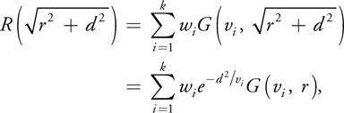
The rendering techniques presented in this chapter use a sum-of-Gaussians formulation. This requires a mapping from a dipole or multipole-based profile to a Gaussian sum. For each diffusion profile R(r), we find k Gaussians with weights w _i and variances v _i such that

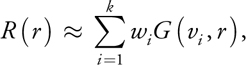
where we choose the following definition for the Gaussian of variance v:

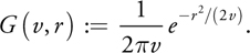
The constant 1/(2v) is chosen such that G(v, r), when used for a radial 2D blur, does not darken or brighten the input image (it has unit impulse response).

Figure 14-12 shows a diffusion profile (for the scattering of green light in marble) and approximations of the profile using two and four Gaussian sums. We use the scattering parameters from Jensen et al. 2001:

a = 0.0041mm-1,

= 2.62mm-1,

= 1.5.

The four-Gaussian sum is

R(r) = 0.070G(0.036, r) + 0.18G(0.14, r) + 0.21G(0.91, r) + 0.29G(7.0, r).

Rendering with the true dipole versus the four-Gaussian sum (using an octree structure following Jensen and Buhler 2002 to ensure accuracy) produces indistinguishable results.

14.4.5 Fitting Predicted or Measured Profiles

This section discusses techniques for approximating a known diffusion profile with a sum of Gaussians. This is not essential to implementing the rendering techniques presented later on, but this section may be useful to readers wishing to accurately approximate subsurface scattering for a material for which they have measured scattering coefficients. Other readers will simply wish to implement the skin shader and interactively experiment with a small number of intuitive parameters (the individual Gaussian weights) to explore the softness of the material, instead of using the parameters computed from scattering theory. We also provide the exact Gaussians used to render all images in this chapter, which should provide a good starting point for rendering Caucasian skin.

The dipole and multipole functions mentioned already can be used to compute diffusion profiles for any material with known scattering coefficients. ^[2] Alternatively, diffusion profiles can be measured from a real-world object by analyzing scattering of laser or structured light patterns (Jensen et al. 2001, Tariq et al. 2006). Once we know exact profiles for the desired material, we must find several Gaussians whose sum matches these profiles closely. We can find these by discretizing the known profile and then using optimization tools (such as those available in Mathematica and MATLAB) that perform the fitting for us. These fitting functions are based on minimizing an error term. If we know a target diffusion profile R(r) with which we want to render, we find k Gaussians that minimize the following:

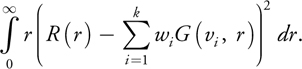
This computes an error function, where a squared error between R(r) and the sum of Gaussians at radial distance r is weighted by r, because the profile at position r gathers light from a circle with circumference proportional to r. Both w_i and v_i for each Gaussian are allowed to vary.

Four Gaussians are sufficient to model most single-layer materials. As an experiment, we have fit four Gaussians to every material profile listed in Jensen et al. 2001, which gives measured parameters for many materials such as milk, marble, ketchup, skin, and more. For each material, we measured error with the following metric

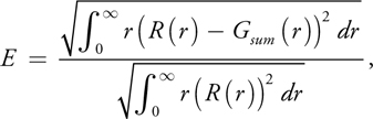
which gives a root-mean-square ratio between the error in fitting R(r) with a sum of Gaussians, G_sum (r), and the target profile itself. The errors ranged from 1.52 percent (for Spectralon, blue wavelength) to 0.0323 percent (for ketchup, green wavelength). Of course, additional Gaussians can be used for increased accuracy and for approximating multilayer materials, which have more complex profiles.

14.4.6 Plotting Diffusion Profiles

Plotting the 1D radial profile and the Gaussian sum that approximates it can help visualize the quality of the fit. We recommend a radially-weighted visualization that plots r x R(r) versus distance, r, as shown previously in Figure 14-12; this weights the importance of a value at radius r based on the circle proportional to radius r to which it is applied during rendering. This has the nice property that the area under the curve is proportional to the total diffuse response (the color reflected when unit white light reflects off the surface). If the fit is poor for r in the range [r ₁, r ₂] but the area under the curve in [r ₁, r ₂] relative to the total area under the curve for all r > 0 is negligible, then errors in the profile at distances [r ₁, r ₂] are also negligible in all but certain contrived lighting scenarios. We can then quickly see whether errors in the fit really matter or not, which is hard to see with standard or logarithmic plots of R(r).

14.4.7 A Sum-of-Gaussians Fit for Skin

Multilayer diffusion profiles can have more complex shapes than dipole profiles, and we found six Gaussians were needed to accurately match the three-layer model for skin given in Donner and Jensen 2005. We use the Gaussian parameters described in Figure 14-13 to match their skin model. The resulting diffusion profiles are shown in Figure 14-14.

Notice here that the Gaussian weights for each profile sum to 1.0. This is because we let a diffuse color map define the color of the skin rather than have the diffusion profiles embed it. By normalizing these profiles to have a diffuse color of white, we ensure that the result, after scattering incoming light, remains white on average. We then multiply this result by a photo-based color map to get a skin tone. We also describe alternative methods for incorporating diffuse color in Section 14.5.2.

Also note that we used the same six Gaussians with the same six variances, and each profile weights them differently. This reduces the amount of shader work required to render with these profiles, and we found that this still produces very good results. However, letting green and blue each fit their own set of six Gaussians would provide more accurate diffusion profiles for green and blue.

With the Gaussian sums that fit our red, green, and blue diffusion profiles, we are ready to render using the new methods presented next. We use the relative weighting of the Gaussians in each sum, as well as the exact variance of each Gaussian in the sum, in our shading system.

14.5 Advanced Subsurface Scattering

This section presents the details of the subsurface scattering component of our skin-rendering system, including our extensions to texture-space diffusion and translucent shadow maps. We compute several blurred irradiance textures and combine them all in the final render pass. One texture is computed for each Gaussian function used in the diffusion profiles. A simple stretch-correction texture enables more accurate separable convolution in the warped UV texture space. We modify the translucent shadow maps technique (Dachsbacher and Stamminger 2004) and combine it with the blurred irradiance textures to allow convincing scattering through thin regions, such as ears.

Using six off-screen blur textures allows accurate rendering with the three-layer skin model as used in Donner and Jensen 2005. We replicate one of their renderings as closely as possible, and show the real-time result in Figure 14-15. The skin color does not match exactly, since the average color of their diffuse map was not specified and their shadow edges are softer due to an area-light source. The real-time result is otherwise very similar to the offline rendering, which required several minutes to compute.

14.5.1 Texture-Space Diffusion

The texture-space diffusion technique introduced by Borshukov and Lewis 2003 for rendering faces in The Matrix sequels can be used to accurately simulate subsurface scattering. Their simple yet powerful insight was to exploit the local nature of scattering in skin and simulate it efficiently in a 2D texture by unwrapping the 3D mesh using texture coordinates as render coordinates. They then model the scattering of light by applying a convolution operation (blur) to the texture, which can be performed very efficiently. The desired shape of the blur is exactly the diffusion profiles of the material (thus requiring different blurs in red, green, and blue). They use a sum of two simple, analytic diffusion profiles: a broad base and a sharp spike (details in Borshukov and Lewis 2005). These two terms approximate the narrow scattering of the epidermis on top of the broadly scattering dermis, but introduce parameters not directly based on any physical model. Adjustment of these parameters is left to an artist and must be tuned by hand. Our sum-of-Gaussians diffusion profile approximations enable faster rendering and produce more accurate scattering since they are derived from physically based models.

Texture-space diffusion extends nicely to GPUs, as shown by Green 2004. We extend Green's implementation in several ways to incorporate transmission through thin regions such as ears (where Borshukov and Lewis used ray tracing) and to improve the accuracy of the results by using stretch correction and better kernels. Previous real-time implementations of texture-space diffusion (Green 2004, Gosselin 2004) use only a single Gaussian kernel (or Poisson-disk sampling), which is only a very rough approximation of true scattering.

14.5.2 Improved Texture-Space Diffusion

We modify texture-space diffusion to provide a more accurate approximation to sub-surface scattering. The new algorithm, executed every frame—illustrated in Figure 14-16—is as follows:

1. Render any shadow maps.
2. Render stretch correction map (optional: it may be precomputed).
3. Render irradiance into off-screen texture.
4. For each Gaussian kernel used in the diffusion profile approximation:
   1. Perform a separable blur pass in U (temporary buffer).
   2. Perform a separable blur pass in V (keep all of these for final pass).
5. Render mesh in 3D:
   1. Access each Gaussian convolution texture and combine linearly.
   2. Add specular for each light source.

Many Blurs

Our first extension of standard texture-space diffusion is to perform many convolution operations to the irradiance texture and to store the results (discarding the temporary buffers used during separable convolutions). We start with the same modified vertex shader in Green 2004 to unwrap the mesh using the texture coordinates as render coordinates. A fragment shader then computes the incoming light from all light sources (excluding specular) to produce the irradiance texture. Figure 14-17 shows an irradiance texture, and also the same texture convolved by the largest Gaussian in our scattering profiles.

Because we fit our diffusion profiles to a sum of six Gaussians, we compute six irradiance textures. The initial, non-blurred irradiance texture is treated as the narrowest Gaussian convolution (because the kernel is so narrow it wouldn't noticeably blur into neighboring pixels), and then we convolve it five times to produce five textures similar to the one in Figure 14-17b. These textures may or may not include diffuse color information, depending on the manner in which diffuse color gets integrated (see upcoming discussion).

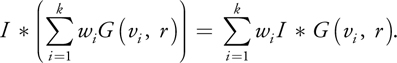
As Figure 14-18 shows, none of the six convolved irradiance textures will generate realistic skin if used alone as an approximation of subsurface scattering. But when blended using the exact same linear combination as was used to fit the six Gaussians to the diffusion profiles of the skin model, they produce the desired appearance. This comes from a convenient property of convolution: the convolution of an image by a kernel that is a weighted sum of functions is the same as a weighted sum of images, each of which is the original image convolved by each of the functions:

Figure 14-19 shows the result of diffusing white light over the face using improved texture-space diffusion with six irradiance textures. No diffuse color texture is used, no specular light is added, and the diffusion profiles are normalized to a white color and then displayed separately in grayscale for red, green, and blue to show the difference in scattering for different wavelengths of light.

Advantages of a Sum-of-Gaussians Diffusion Profile

We could directly convolve the irradiance texture by a diffusion profile using a one-pass 2D convolution operation (as is done by Borshukov and Lewis 2003). However, this would be quite expensive: we store an average of 4 samples (texels) per millimeter on the face in the irradiance texture, and the width of the diffusion profile for red light would be about 16 mm, or 64 texels. Thus, we would need a 64 x 64 or 4,096-tap blur shader. If the diffusion profile was separable we could reduce this to only a 64 + 64 or 128-tap blur. But diffusion profiles are radially symmetric because we assume a homogeneous material that scatters light equally in all directions, and therefore they are not separable, for Gaussians are the only simultaneously separable and radially symmetric functions and we have seen that diffusion profiles are not Gaussians.

However, each Gaussian convolution texture can be computed separably and, provided our fit is accurate, the weighted sum of these textures will accurately approximate the lengthy 2D convolution by the original, nonseparable function. This provides a nice way to accelerate general convolutions by nonseparable functions: approximate a nonseparable convolution with a sum of separable convolutions. We use this same idea to accelerate a high-dynamic-range (HDR) bloom filter in Section 14.6.

Another nice property of Gaussians is that the convolution of two Gaussians is also a Gaussian. This allows us to generate each irradiance texture by convolving the result of the previous one, in effect allowing us to convolve the original image by wider and wider Gaussians without increasing the number of taps at each step. Two radial Gaussians with variances v ₁ and v ₂ convolve into the following

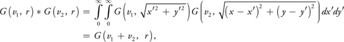
where G is the Gaussian defined on page 309 and r = . Thus, if the previous irradiance texture contains I * G(v ₁, r) (where I is irradiance) and we wish to compute I * G(v ₂, r), we simply convolve with G(v ₂ - v ₁, r).

We use a seven-tap, separable convolution shader and store the intermediate result of convolution in the U direction to a temporary buffer before convolving in V. The seven Gaussian taps are {0.006, 0.061, 0.242, 0.383, 0.242, 0.061, 0.006}. This represents a Gaussian with a standard deviation of 1.0, assuming the coordinates of the taps are {-3.0, -2.0, -1.0, 0.0, 1.0, 2.0, 3.0}. This seven-tap kernel is used for all convolution steps, and the taps are linearly scaled about the center tap to convolve by any desired Gaussian. (The spacing should be scaled by the square root of the variance—the standard deviation—of the desired Gaussian.) Successive kernel widths in a sum-of-Gaussians fit should never be more than about twice the previous width. Doing so would increase the error from the use of stretch-correction values (presented in the next section) and would require more than seven samples in later convolution steps to prevent under-sampling. In our experience, fitting several Gaussians to a diffusion profile invariably gives a set of widths in which each is roughly double the last (variance changes by roughly 4x), and thus using seven taps at every step works well.

To summarize, we perform six 7-tap separable convolutions, for a total of 6 x 2 x 7 = 84 texture accesses per output texel instead of the 4,096 required to convolve with the original diffusion profile in one step.

Correcting for UV Distortion

If the surface is flat and the convolution kernels used to blur the irradiance are exactly the diffusion profiles of the material, then texture-space diffusion is very accurate. However, some issues arise when this technique is applied to curved surfaces.

On curved surfaces, distances between locations in the texture do not correspond directly to distances on the mesh due to UV distortion. We need to address UV distortion to more accurately handle convolution over curved surfaces. Using simple stretch values that can be computed quickly every frame we have found it possible to correct for this (to a large degree), and the results look very good, especially for surfaces like faces which do not have extreme curvature. Ignoring UV distortion can cause a red glow around shadows and can produce waxy-looking diffusion in regions such as ears, which are typically more compressed in texture space compared to other surface regions.

We compute a stretch-correction texture that modulates the spacing of convolution taps for each location in texture space, as shown in Figure 14-20. The resulting width of convolution is roughly the same everywhere on the mesh (and therefore varies across different regions of the texture). We compute stretching in both the U and V texture-space directions, since horizontal and vertical stretching usually differ significantly.

We compute the stretch-correction texture using a simple fragment shader, presented in Listing 14-4. We reuse the same vertex shader used to unwrap the head into texture space for computing the irradiance texture, and store the world-space coordinates of the mesh in a texture coordinate. Screen-space derivatives of these coordinates give efficient estimates of the stretching, which we invert and store in the stretch-correction texture. The same values are accessed later in the convolution shaders (Listing 14-5) for directly scaling the spread of convolution taps.

Example 14-4. Computing a Two-Component Stretch Texture

The stretch texture is computed very efficiently and can be computed per frame for highly deforming meshes. Texture-space derivatives of world-space coordinates give an accurate estimate of local stretching, which is inverted and directly multiplied by blur widths later. A constant may be needed to scale the values into the [0,1] range.

    float2 computeStretchMap( float3 worldCoord : TEXCOORD0 ) {   float3 derivu = ddx( worldCoord );   float3 derivv = ddy( worldCoord );   float stretchU = 1.0 / length( derivu );   float stretchV = 1.0 / length( derivv );   return float2( stretchU, stretchV ); // A two-component texture } 

The Convolution Shader

Listing 14-5 is used to convolve each texture in the U direction. An analogous convolveV() shader is used for the second half of a separable convolution step.

Optional: Multiscale Stretching

The stretch maps will have a constant value across each triangle in the mesh and thus will be discontinuous across some triangle edges. This should not be a problem for very small convolutions, but high-frequency changes in stretch values could cause high-frequency artifacts for very large convolutions. The derivatives used to compute stretching consider two neighboring texels, and thus the values may be poor estimates of the average stretching over a width of, say, 64 texels.

A more general approach is to duplicate the convolution passes used to convolve irradiance and convolve the stretch maps as well. Then use the kth convolution of the stretch map to convolve the kth irradiance texture. The idea here is to select a stretch map that has locally averaged the stretching using the same radius you are about to convolve with, and use that average value to correct the current convolution of irradiance.

Example 14-5. A Separable Convolution Shader (in the U Texture Direction)

The final spacing of the seven taps is determined by both the stretch value and the width of the desired Gaussian being convolved with.

    float4 convolveU( float2 texCoord : TEXCOORD0,   // Scale – Used to widen Gaussian taps.    // GaussWidth should be the standard deviation.    uniform float GaussWidth,   // inputTex – Texture being convolved    uniform texobj2D inputTex,   // stretchTex - Two-component stretch texture    uniform texobj2D stretchTex ) {   float scaleConv = 1.0 / 1024.0;   float2 stretch = f2tex2D( stretchTex, texCoord );   float netFilterWidth = scaleConv * GaussWidth * stretch.x;   // Gaussian curve – standard deviation of 1.0    float curve[7] = {0.006,0.061,0.242,0.383,0.242,0.061,0.006};   float2 coords = texCoord - float2( netFilterWidth * 3.0, 0.0 );   float4 sum = 0;   for( int i = 0; i < 7; i++ )   {     float4 tap = f4tex2D( inputTex, coords );     sum += curve[i] * tap;     coords += float2( netFilterWidth, 0.0 );   }   return sum; } 

The Accuracy of Stretch-Corrected Texture-Space Diffusion

Figure 14-21 shows artifacts that arise from convolving in texture space without correcting for stretching, and the degree to which they are corrected using static and multiscale stretch maps. A spatially uniform pattern of squares is projected onto a head model and convolved over the surface in texture space. We show convolution by three Gaussians of varying widths. The left images use no stretching information and exhibit considerable artifacts, especially for the wide convolutions. In the center images, the results are greatly improved by using a single, static stretch map (used for all convolutions of any size).

Multiscale stretch correction (right) does not improve the results dramatically for the face model, and a single, static map is probably sufficient. However, when we render more complicated surfaces with very high distortions in texture space, multiscale stretch correction may prove noticeably beneficial. Further accuracy may be achieved by using the most conformal mapping possible (and possibly even locally correcting convolution directions to be nonorthogonal in texture space to ensure orthogonality on the mesh).

Incorporating Diffuse Color Variation

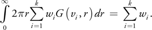
Diffusion profiles implicitly determine the net diffuse color of a material. Consider, again, the laser dot experiment. If a focused white laser light illuminates a surface and the total amount of light reflected back (considering every point on the surface) is less than (1, 1, 1) (that is, unit white light), then some of the light is absorbed by the surface. The total reflected amount, (r, g, b), is the diffuse color of the material (or the total diffuse reflectance R_d ). This can be computed for known diffusion profiles by integrating over all distances r > 0. Each distance r corresponds to light reflected at a circle of radius 2r, giving the following:

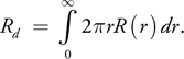
This is trivial to compute for a profile expressed as a sum of Gaussians: R_d is simply the sum of the weights in the Gaussian sum (the constant factor in our Gaussian definition was chosen to achieve this result):

Dipole and multipole theories assume a homogeneous material, perfectly uniform over the plane, and thus predict a perfectly constant skin color everywhere, R_d . However, skin has both high-frequency and low-frequency variation in color, which we would like to model. Physically this corresponds to nonuniformities in the different layers of skin that cause the scattering and absorption properties to vary within the tissue layers. This is currently impractical to simulate in real time (and it's not even clear how to measure these variations, especially within living tissue), so we resort to using textures to simulate the effects of this much more complicated process.

Diffuse color maps can be generated from photographs or painted by an artist and are an obvious way to control color variation across the skin surface. The color maps used in this chapter were made directly from photographs of a real person under diffuse illumination (white light arriving equally from all directions). Multiple photos were projected onto a single mesh and combined into a single texture.

We can choose among several ways to incorporate diffuse color maps into our scattering model. Since the model was derived assuming a perfectly uniform material, none of these techniques is completely physically based, and each may prove useful in different scenarios.

Post-Scatter Texturing

One option is to first perform all scattering computations without any coloring producing a value that everywhere averages to white, and then multiply by the diffuse color map to get the desired skin tone. The diffusion profile is normalized to white by using the code in Listing 14-6, which divides each Gaussian weight by the sum of all weights. Diffuse color is not used in the irradiance texture computation. The resulting scattered light is thus white on average (or, to be more exact, the color of the incoming light), and the final linear combination of all irradiance textures looks like Figure 14-22 (top right). The diffuse color texture is multiplied after scattering: the result is shown in Figure 14-22 (bottom right) (specular was also added). All the high-frequency texture detail is maintained because it is not blurred by the convolution passes, but no color bleeding of the skin tones occurs, which may make this option undesirable. However, if the diffuse map came from photographs of real skin, natural color bleeding has already occurred, and performing extra blurring may not be appropriate, so this post-scatter texturing may be the best alternative. The images in this chapter of the Adrian data set from XYZ RGB, Inc. (shown previously in Figure 14-15) are rendered with post-scatter texturing.

Donner and Jensen 2005 suggest also convolving the diffuse color map using the exact same profiles with which irradiance is convolved, to achieve proper color bleeding, and then multiplying this convolved color value by the convolved irradiance (which is convolved separately). This is slightly different from the next option, pre-scatter texturing. One is the convolution of a product; the other, a product of convolutions, and either may look better, depending on the diffuse map used.

Pre-Scatter Texturing

Another way to incorporate diffuse color variation is pre-scatter texturing. The lighting is multiplied by the diffuse color when computing the irradiance texture and then not used in the final pass. This scatters the diffuse color the same way the light is scattered, blurring it and softening it, as shown in Figure 14-22 (bottom left).

A possible drawback to this method is that it may lose too much of the high-frequency detail such as stubble, which sits at the top of the skin layers and absorbs light just as it is exiting. However, a combination of the two techniques is easy to implement and offers some color bleeding while retaining some of the high-frequency details in the color map.

Combining Pre-Scatter and Post-Scatter Texturing

A portion of the diffuse color can be applied pre-scatter and the rest applied post-scatter. This allows some of the color detail to soften due to scattering, yet it allows some portion to remain sharp. Because the diffuse color map contains the final desired skin tone, we can't multiply by diffuseColor twice. Instead, we can multiply the lighting by pow(diffuseColor, mix) before blurring and multiply the final combined results of all blurred textures by pow(diffuseColor, 1 – mix). The mix value determines how much coloring applies pre-scattering and post-scattering, and the final skin tone will be the desired diffuseColor value. A mix value of 0.5 corresponds to an infinitesimal absorption layer on the very top of the skin surface that absorbs light exactly twice: once as it enters before scattering, and once as it leaves. This is probably the most physically plausible of all of these methods and is the technique used in Weyrich et al. 2006.

The images of Doug Jones in this chapter (such as Figure 14-1) use a mix value of 0.5. However, other values may look better, depending on the diffuse color texture and how it was generated. When using a mix value of exactly 0.5, replace the pow(diffuse-Color, 0.5) instructions with sqrt(diffuseColor) for better performance.

Compute Specular and Diffuse Light with the Same Normals

One approximation to subsurface scattering mimics the softening of diffuse lighting by using different normal maps (or bump height/displacement maps) for computing specular versus diffuse lighting (or even separate maps for each of red, green, and blue diffuse lighting, as described in Ma et al. 2007). Specular lighting reflects directly off the surface and isn't diffused at all, so it shows the most dramatic, high-frequency changes in the skin surface. The remaining (nonspecular) lighting is diffused through the skin, softening the high-frequency changes in lighting due to surface detail—bumps, pores, wrinkles, and so on—with red light diffusing farthest through the skin's subsurface layers and softening the most. However, simply blurring normal maps does not correctly diffuse the skin tones or the actual lighting itself. Because the methods we present in this chapter directly model the subsurface scattering responsible for the softening of surface details, the true normal information should be used for both specular and diffuse computations.

The Final Shader

Listing 14-6 gives the fragment shader for the final render pass. The mesh is rendered in 3D using a standard vertex shader. Gaussian weights that define the diffusion profiles are input as float3 constants (x for red, y for green, and z for blue). These should be the values listed in Figure 14-13 so that the mixing of the blurred textures matches the diffusion profiles. The Gaussian weights are renormalized in the shader allowing them to be mapped to sliders for interactive adjustment. Raising any Gaussian weight automatically lowers the other five to keep the total at 1.0. Thus the final diffuse light is not brightened or darkened, but the ratio of broad blur to narrow blur is changed; this will change the softness of the skin and is a convenient way to interactively edit the final appearance. This may be necessary for achieving skin types for which exact scattering parameters are not know, or for which the game or application demands a particular "look" rather than photorealism, but we have found that the three-layer model in Donner and Jensen 2005 works well for realistic Caucasian skin and we do not modify the weights at all.

Example 14-6. The Final Skin Shader

    float4 finalSkinShader(float3 position : POSITION,   float2 texCoord : TEXCOORD0,   float3 normal : TEXCOORD1,   // Shadow map coords for the modified translucent shadow map    float4 TSM_coord : TEXCOORD2,   // Blurred irradiance textures    uniform texobj2D irrad1Tex,   . . .   uniform texobj2D irrad6Tex,   // RGB Gaussian weights that define skin profiles    uniform float3 gauss1w,   . . .   uniform float3 gauss6w,   uniform float mix, // Determines pre-/post-scatter texturing    uniform texobj2D TSMTex,   uniform texobj2D rhodTex ) {   // The total diffuse light exiting the surface    float3 diffuseLight = 0;   float4 irrad1tap = f4tex2D( irrad1Tex, texCoord );   . . .   float4 irrad6tap = f4tex2D( irrad6Tex, texCoord );   diffuseLight += gauss1w * irrad1tap.xyz;   . . .   diffuseLight += gauss6w * irrad6tap.xyz;   // Renormalize diffusion profiles to white    float3 normConst = gauss1w + guass2w + . . . + gauss6w;   diffuseLight /= normConst; // Renormalize to white diffuse light    // Compute global scatter from modified TSM    // TSMtap = (distance to light, u, v)    float3 TSMtap = f3tex2D( TSMTex, TSM_coord.xy / TSM_coord.w ); // Four average thicknesses through the object (in mm)    float4 thickness_mm = 1.0 * -(1.0 / 0.2) *                       log( float4( irrad2tap.w, irrad3tap.w,                                    irrad4tap.w, irrad5tap.w )); float2 stretchTap = f2tex2D( stretch32Tex, texCoord ); float stretchval = 0.5 * ( stretchTap.x + stretchTap.y ); float4 a_values = float4( 0.433, 0.753, 1.412, 2.722 ); float4 inv_a = -1.0 / ( 2.0 * a_values * a_values ); float4 fades = exp( thickness_mm * thickness_mm * inv_a ); float textureScale = 1024.0 * 0.1 / stretchval; float blendFactor4 = saturate(textureScale *                               length( v2f.c_texCoord.xy - TSMtap.yz ) /                               ( a_values.y * 6.0 ) ); float blendFactor5 = saturate(textureScale *                               length( v2f.c_texCoord.xy - TSMtap.yz ) /                               ( a_values.z * 6.0 ) ); float blendFactor6 = saturate(textureScale *                               length( v2f.c_texCoord.xy - TSMtap.yz ) /                               ( a_values.w * 6.0 ) ); diffuseLight += gauss4w / normConst * fades.y * blendFactor4 *                 f3tex2D( irrad4Tex, TSMtap.yz ).xyz; diffuseLight += gauss5w / normConst * fades.z * blendFactor5 *                 f3tex2D( irrad5Tex, TSMtap.yz ).xyz; diffuseLight += gauss6w / normConst * fades.w * blendFactor6 *                 f3tex2D( irrad6Tex, TSMtap.yz ).xyz; // Determine skin color from a diffuseColor map diffuseLight *= pow(f3tex2D( diffuseColorTex, texCoord ), 1.0–mix); // Energy conservation (optional) – rho_s and m can be painted    // in a texture    float finalScale = 1 – rho_s*f1tex2D(rhodTex, float2(dot(N, V), m); diffuseLight *= finalScale; float3 specularLight = 0;   // Compute specular for each light    for (each light)     specularLight += lightColor[i] * lightShadow[i] *                 KS_Skin_Specular( N, L[i], V, m, rho_s, beckmannTex );   return float4( diffuseLight + specularLight, 1.0 ); } 

Dealing with Seams

Texture seams can create problems for texture-space diffusion, because connected regions on the mesh are disconnected in texture space and cannot easily diffuse light between them. Empty regions of texture space will blur onto the mesh along each seam edge, causing artifacts when the convolved irradiance textures are applied back onto the mesh during rendering.

An easy solution is to use a map or alpha value to detect when the irradiance textures are being accessed in a region near a seam (or even in empty space). When this is detected, the subsurface scattering is turned off and the diffuse reflectance is replaced with an equivalent local-light calculation. A lerp makes this transition smooth by blending between scattered diffuse light and nonscattered diffuse light (the alpha map is pre-blurred to get a smooth lerp value). Also, painting the stretch textures to be black along all seam edges causes the convolution kernels to not blur at all in those regions, reducing the distance from the seam edges at which the scattering needs to be turned off. This solution creates hard, dry-looking skin everywhere the object contains a seam, and may be noticeable, but it worked well for the NVIDIA "Froggy" and "Adrianne" demos. For the head models shown in this chapter the UV mappings fill the entire texture space, so none of these techniques are required. Objectionable seams are visible only under very specific lighting setups.

A more complicated solution involves duplicating certain polygons of the mesh for the irradiance texture computation. If there is sufficient space, all polygons that lie against seam-edges are duplicated and placed to fill up the empty texture space along seam edges. If light never scatters farther than the thickness of these extra polygons, then empty space will never diffuse onto accessed texels and light will properly scatter across seam edges. These extra polygons are rendered only in the irradiance texture pass and not in the final render pass. The duplicated polygons may need to overlap in a small number of places in the texture, but this should not create significant artifacts. We expect this technique would provide a good solution for many meshes, but have not tried it ourselves.

A more general solution is to find many overlapping parameterizations of the surface such that every point is a safe distance away from seam edges in at least one texture. The irradiance texture computation and convolution passes are duplicated for each parameterization (or many parameterizations are stored in the same texture) and a partition of unity—a set of weights, one for each parameterization—blends between the different sets of textures at every location on the surface. This "turns off" bad texture coordinates in locations where seam edges are near and "turns on" good ones. These weights should sum to 1.0 everywhere and vary smoothly over the surface. For each surface location, all weights that are nonzero should correspond to texture parameterizations that are a safe distance away from seam edges. Techniques for computing such parameterizations and their respective partitions of unity can be found in Piponi and Borshukov 2000. Given a partition of unity, the entire texture-space diffusion algorithm is run for each parameterization and the results are blended using the partition weights. This requires a considerable amount of extra shading and texture memory and is comparatively expensive, but probably still outperforms other subsurface-scattering implementations.

Exact Energy Conservation

Specular reflectance and diffuse reflectance are often treated completely independently, regardless of incoming and outgoing angles. This approach ignores a subtle interplay between the two from an energy standpoint, for if the specular reflections (not just for a single view direction, but over the entire hemisphere of possible view directions) consume, say, 20 percent of all incoming light, no more than 80 percent is left for diffuse. This seems fine, because shading is often computed as Ks * specular + Kd * diffuse, where Ks and Kd are constants. But the total amount of energy consumed by specular reflectance is highly dependent on the angle between N and L, and a constant mix of the two does not conserve energy. This topic has been addressed in coupled reflection models such as Ashikmin and Shirley 2000 and Kelemen and Szirmay-Kalos 2001, and it has also been addressed for subsurface scattering in Donner and Jensen 2005. The non-Lambertian diffuse lighting that results is easy to compute on GPUs. Because we are rendering skin we discuss only the subsurface-scattering version here.

The energy available for subsurface scattering is exactly all energy not reflected directly by the specular BRDF. A single specular calculation gives the portion of total input energy reflecting in a single outgoing direction (one L direction, one V direction). To sum the total energy used by specular reflection, all V directions must be considered. Thus, before storing light in the irradiance texture, we need to integrate specular reflectance over all directions on the hemisphere and multiply diffuse light by the fraction of energy that remains. If f_r is the specular BRDF and L is the light vector at position x on the surface, then we attenuate diffuse lighting for each light by the following

Equation 1

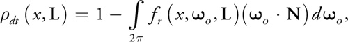
where _o are vectors in the hemisphere about N.

Using spherical coordinates, the integral in Equation 1 is computed as

Equation 2

This value will change depending on roughness m at position x, and on N · L. We remove the _s constant from the specular BRDF (because it can be applied as a constant factor later) and precompute the integral in Equation 2. We precompute it for all combinations of roughness values and angles and store it in a 2D texture to be accessed based on m and N · L. This precomputation is easily performed in the fragment shader given in Listing 14-7. This is only a rough estimate of the 2D integral, because of the uniform sampling, and better numerical integration techniques could also be used on the CPU or GPU to compute this texture. The uniform sample integration is especially poor for low roughness values, as seen in Figure 14-23, but such low values are not used by our skin shader.

Example 14-7. A Fragment Shader for Preintegrating a Specular BRDF over the Hemisphere

The resulting scalar texture is used to retrieve _dt terms when computing accurate subsurface scattering within rough surfaces.

    float computeRhodtTex( float2 tex : TEXCOORD0 ) {   // Integrate the specular BRDF component over the hemisphere    float costheta = tex.x;   float pi = 3.14159265358979324;   float m = tex.y;   float sum = 0.0;   // More terms can be used for more accuracy    int numterms = 80;   float3 N = float3( 0.0, 0.0, 1.0 );   float3 V = float3(0.0, sqrt( 1.0 - costheta*costheta ), costheta);   for( int i = 0; i < numterms; i++ )   {     float phip = float(i) / float( numterms - 1 ) * 2.0 * pi;     float localsum = 0.0f;     float cosp = cos( phip );     float sinp = sin( phip );     for( int j = 0; j < numterms; j++ )     {       float thetap = float(j) / float( numterms - 1 ) * pi / 2.0;       float sint = sin( thetap );       float cost = cos( thetap );       float3 L = float3( sinp * sint, cosp * sint, cost );       localsum += KS_Skin_Specular( V, N, L, m, 0.0277778 ) * sint;     }     sum += localsum * (pi / 2.0) / float( numterms );   }   return sum * (2.0 * pi) / ( float( numterms ) ); } 

This _dt texture can then be used to modify diffuse lighting calculations using the code in Listing 14-8. This is executed for each point or spotlight when generating the irradiance texture. Environment lights have no L direction and should technically be multiplied by a constant that is based on a hemispherical integral of _dt , but because this is just a constant (except for variation based on m) and probably close to 1.0, we don't bother computing this. The correct solution would be to convolve the original cube map using the _dt directional dependence instead of just with N · L.

Example 14-8. Computing Diffuse Irradiance for a Point Light

    float ndotL[i] = dot( N, L[i] ); float3 finalLightColor[i] = LColor[i] * LShadow[i]; float3 Ldiffuse[i] = saturate( ndotL[i] ) * finalLightColor[i]; float3 rho_dt_L[i] = 1.0 - rho_s*f1tex2D(rhodTex, float2(ndotL[i], m)); irradiance += Ldiffuse[i] * rho_dt_L[i]; 

After light has scattered beneath the surface, it must pass through the same rough interface that is governed by a BRDF, and directional effects will come into play again. Based on the direction from which we view the surface (based on N · V), a different amount of the diffuse light will escape. Because we use a diffusion approximation, we can consider the exiting light to be flowing equally in all directions as it reaches the surface. Thus another integral term must consider a hemisphere of incoming directions (from below the surface) and a single outgoing V direction. Because the physically based BRDF is reciprocal (that is, the light and camera can be swapped and the reflectance will be the same) we can reuse the same _dt term, this time indexed based on V instead of L. The end of Listing 14-6 shows how this attenuation is computed.

Failing to account for energy conservation in the scattering computation can lead to overly bright silhouette edges. The effect is subtle but noticeable, especially for skin portrayed against a dark background where it appears to "glow" slightly (see Figure 14-24). Adding energy conservation using our precomputed rho_dt texture provides more realistic silhouettes, but the same effect can unnaturally darken regions such as the edge of the nose in Figure 14-24. Again, the effect is subtle but perceptible. In fact, this darkening represents another failure to conserve energy, this time in a different guise: since we do not account for interreflection, our model misses the light that should be bouncing off the cheekbone region to illuminate the edge of the nose. Precomputed radiance transfer (PRT) techniques can capture such interreflections, but do not support animated or deformable models and thus don't easily apply to human characters. Since the "glow" artifact tends to cancel out the "darkening" effect, but produces its own artifacts, you should evaluate the visual impact of these effects in your application and decide whether to implement energy conservation in the scattering computation.

14.5.3 Modified Translucent Shadow Maps

Texture-space diffusion will not capture light transmitting completely through thin regions such as ears and nostrils, where two surface locations can be very close in three-dimensional space but quite distant in texture space. We modify translucent shadow maps (TSMs) (Dachsbacher and Stamminger 2004) in a way that allows a very efficient estimate of diffusion through thin regions by reusing the convolved irradiance textures.

Instead of rendering z, normal, and irradiance for each point on the surface nearest the light (the light-facing surface), as in a traditional translucent shadow map, we render z and the (u, v) coordinates of the light-facing surface. This allows each point in shadow to compute a thickness through the object and to access the convolved irradiance textures on the opposite side of the surface, as shown in Figure 14-25.

We analyze the simple scenario depicted in Figure 14-26 to see how to compute global scattering. A shadowed point C being rendered needs to sum the scattered light from all points in a neighborhood of point A on the other side of the object. This is typically computed by sampling points around A (on the 2D light-facing surface) and computing the reflectance ^[3] profile R(m), where m is the true distance from C to each point near A.

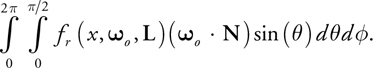
We can use a modified TSM and the convolved irradiance textures to estimate this global transmitted light. At any shadowed location C, the TSM provides the distance m and the UV coordinates of point A on the light-facing surface. We want to estimate the scattered light exiting at C, which is the convolution of the light-facing points by the profile R, where distances from C to each sample are computed individually. Computing this for B, however, turns out to be much easier, and for small angles , B will be close to C. For large , Fresnel and N · L terms will cause the contribution to be small and hide most of the error. Computing the correct value at C is probably not worth the considerable cost.

Computing scattering at B, any sample at distance r away from A on the light-facing surface needs to be convolved by the following

where we have used the separability of Gaussians in the third dimension to transform a function of into a function of r. This is convenient since the light-facing points have already been convolved by G(v_i , r) at A (this is what we store in each of the convolved irradiance textures). Thus the total diffuse light exiting at location C (estimated at B instead) is a sum of k texture lookups (using the (u, v) for location A stored in the TSM), each weighted by w_i and an exponential term based on v_i and d. This transformation works because each Gaussian in the sum-of-Gaussians diffusion profile is separable. A single 2D convolution of light-facing points by the diffusion profile R(r) could not be used for computing scattering at B or C (only at A).

Depths, m, computed by the shadow map are corrected by cos() because a diffusion approximation is being used and the most direct thickness is more applicable. Surface normals at A and C are compared, and this correction is applied only when the normals face opposite directions. A simple lerp blends this correction back to the original distance m as the two normals approach perpendicular. Although derived in a planar setting, this technique tends to work fairly well when applied to nonplanar surfaces such as ears (as shown in Figure 14-27).

So far we have considered only one path of light through the object, which can lead to some problems. High-frequency changes in depth computed from the TSM can lead to high-frequency artifacts in the output. This is undesirable for highly scattering translucence, which blurs all transmitted light and should have no sharp features. A useful trick to mask this problem is to store depth through the surface in the alpha channel of the irradiance texture and blur it over the surface along with irradiance. Each Gaussian, when computing global scattering, uses a corresponding blurred version of depth. (We use the alpha of texture i - 1 for the depth when computing Gaussian i.) This allows each ray through the object to consider the average of a number of different paths, and each Gaussian can choose an average that is appropriate. To pack the distance value into an 8-bit alpha, we store exp(-const * d) for some constant, d, convolve this exponential of depth over the surface, and reverse after lookup. See Listing 14-9.

Example 14-9. Computing the Irradiance Texture

Depth through the surface is stored in the alpha channel and is convolved over the surface.

    float4 computeIrradianceTexture() {   float distanceToLight = length( worldPointLight0Pos – worldCoord );   float4 TSMTap = f4tex2D( TSMTex, TSMCoord.xy / TSMCoord.w );   // Find normal on back side of object, Ni    float3 Ni = f3tex2D( normalTex, TSMTap.yz ) * float3( 2.0, 2.0, 2.0 ) -               float3( 1.0, 1.0, 1.0 );   float backFacingEst = saturate( -dot( Ni, N ) );   float thicknessToLight = distanceToLight - TSMTap.x;   // Set a large distance for surface points facing the light    if( ndotL1 > 0.0 )   {     thicknessToLight = 50.0;   }   float correctedThickness = saturate( -ndotL1 ) * thicknessToLight;   float finalThickness = lerp( thicknessToLight, correctedThickness,                                backFacingEst );   // Exponentiate thickness value for storage as 8-bit alpha    float alpha = exp( finalThickness * -20.0 );   return float4( irradiance, alpha ); } 

Double contribution can occur when the (u, v) of the point being rendered approaches the (u, v) of the point in the TSM. We lerp the TSM contribution to 0 for each Gaussian term as the two (u, v) coordinates approach each other. This is done using the blendFactor terms in Listing 14-6.

Figure 14-27 shows two renders using this technique, one where the distance correction is not used, and another where it is. Figure 14-28 shows the local scattering and then each individual Gaussian global scatter term separately. When summed, these four images give the final image in Figure 14-27 (right).

Multiple Lights and Environment Lighting

The extended TSM technique was derived assuming a single point light with a single TSM. Using many TSMs requires creating convolved irradiance textures for each light and storing them separately. (Each TSM needs an associated set of convolved irradiance textures for that light only.) This requires many extra blur passes and extra texture memory. A possible way around this is to compute the minimum of all depths through the surface (using multiple TSMs) and convolve that over the surface. In the final shader, each TSM can be accessed, and the (u, v) corresponding to the smallest of all computed thicknesses can be used to do a single TSM global scatter computation. This is certainly an approximation, but it avoids scaling the entire texture-space diffusion algorithm by the number of point light sources.

In general, we have found modified translucent shadow maps to work well for dramatic lighting (Figure 14-27), but it still leaves ears looking somewhat opaque with bright environment lighting. This is a common phenomenon for offline rendering as well and has been addressed in Donner and Jensen 2007. The solution is rather expensive, and no real-time approximation is immediately obvious.

14.6 A Fast Bloom Filter

The same techniques used to accelerate convolutions for subsurface scattering apply in general to other nonseparable convolutions, such as bloom filters. Pharr and Humphreys 2004 recommend a bloom filter of (1 - r/d)⁴ for adding bloom to a final rendered image (especially nice for HDR images). This filter is not separable and must be computed brute-force in 2D. However, it is well approximated by a sum of two Gaussians, and the same separable, hierarchical convolution techniques used for improved texture-space diffusion (excluding the stretch textures) can be used to efficiently evaluate it. For d = 1, (1 - r)⁴ is well approximated by 0.0174 G(0.008, r) + 0.192 G(0.0576, r). Figure 14-29 shows an image with skin rendering and an HDR bloom filter computed using this two-Gaussian kernel.

14.7 Conclusion

Our new sum-of-Gaussians formulation of diffusion profiles makes possible new algorithms based on texture-space diffusion and translucent shadow maps that produce highly realistic real-time images of human skin. Physically based multilayer skin models map directly to these new algorithms, enabling us to demonstrate real-time renderings with a level of realism attained previously only in offline rendering. See Figure 14-29 for a final example.

Real-time imagery such as Figure 14-29 will consume most of the resources of an entire GeForce 8800 Ultra GPU. However, the techniques presented in this chapter are somewhat scalable and the texture resolutions can be greatly reduced for characters that do not fill the entire screen. Using fewer than six Gaussians to approximate diffusion profiles will likely suffice for most characters. Subsurface scattering becomes less noticeable in very far away characters, and a level-of-detail system should be able to move between multiple levels of diffusion accuracy without noticeable popping.

We were greatly inspired by the groundbreaking work of Craig Donner and Henrik Wann Jensen in 2005, and hopefully, like us, readers will be inspired to approximate these and future results as closely as they can—as their applications permit—and create the most realistic real-time characters possible.

14.7.1 Future Work

Although this chapter focuses on real-time face rendering, many of the techniques apply to a wide variety of materials with highly scattering translucence. We expect that the subsurface-scattering algorithms we have developed for efficient GPU rendering may also prove useful in an offline rendering pipeline.

The skin-rendering techniques we presented work wonderfully for faces, but texture seams pose difficulties for rendering general surfaces, especially hands and feet. The solutions discussed for addressing seams need to be explored in more detail to determine to what extent they can be addressed automatically with no user input (which might make the texture-space diffusion idea more viable for general-purpose rendering), and to test the applicability of improved texture-space diffusion to more general rendering of translucent materials.

Correcting texture-space convolution kernels based on multiscale normal curvature proved negligible for face rendering, but improvements such as this and multiscale stretch correction should be explored further to determine the degree to which texture-space diffusion can generate realistic images of subsurface scattering as the surface curvatures become comparable to the effective radius of scattering. Donner and Jensen 2007 presents a more accurate solution for diffuse scattering in curved surfaces and their results should be considered when improving real-time scattering techniques.

For skin rendering in general, the spectral bidirectional surface-scattering reflectance distribution function (BSSRDF) model by Donner and Jensen 2006 and the five-layer BioSpec model (Krishnaswamy and Baranoski 2004) should provide more accurate images, but exact comparisons between these models and the three-layer skin model in Donner and Jensen 2005 have not been generated. It is not clear what visual impact these more physically accurate models have. In particular, a study comparing spectral skin rendering with varying numbers of color bands in the range of 3–150 would be telling. An exact-as-possible comparison of the Donner and Jensen diffusion models to a full Monte-Carlo, ground-truth simulation based on the BioSpec model should also reveal the impact of the simplification of using two or three layers instead of five, as well as what is lost in assuming a diffusion approximation.

Single scattering is often ignored for subsurface-scattering simulations and in particular for skin rendering. Methods from Hanrahan and Krueger 1993 are not directly applicable due to the rough surface layer, which turns a single-scattering process into a triple-scattering process. The extent to which this directional component of subsurface scattering matters could be studied using Monte Carlo methods. If significant at grazing angles, this component could potentially be modeled as a BRDF or BSSRDF by decoupling subsurface irradiance into diffuse and single-scattering. A physically based bidirectional transmittance distribution function (BTDF) (Stam 2001) for the epidermis based on a model of the cells in the stratum corneum—the outermost layer of the epidermis—should provide the best data.

Incorporating variation in skin color still remains a rather ad hoc process. Future work for capturing, incorporating, and editing skin color variation with predictably good results would be very beneficial. Anisotropy and varying scattering coefficients over different facial regions were noted in Weyrich et al. 2006 and Tariq et al. 2006. A fast-capture system for capturing spatially varying diffusion profiles with multilayered fidelity over a face could also potentially improve images.

Asperity scattering (Koenderink and Pont 2003) has not been modeled and should be incorporated to simulate scattering from hairs on the face.

The Torrance/Sparrow specular BRDF might be improved by using a model fit to real-world measurements of real skin reflectance or to a simulation of surface scattering based on a physically based model of the cells in the stratum corneum. One such BTDF model is used in BioSpec. The polarization techniques from Debevec et al. 2000 should allow direct measurement of the exact specular-only BRDF for real skin.

14.8 References

Ashikmin, Michael, and Peter Shirley. 2000. "An Anisotropic Phong Light Reflection Model." Technical report UUCS-00-014, University of Utah.

Borshukov, George, and J. P. Lewis. 2003. "Realistic Human Face Rendering for The Matrix Reloaded." In ACM SIGGRAPH 2003 Sketches and Applications.

Borshukov, George, and J. P. Lewis. 2005. "Fast Subsurface Scattering." In ACM SIGGRAPH 2005 Course on Digital Face Cloning.

d'Eon, Eugene. 2007. "NVIDIA Demo Team Secrets–Advanced Skin Rendering." Presentation at Game Developer Conference 2007. Available online at http://developer.download.nvidia.com/presentations/2007/gdc/Advanced_Skin.pdf.

d'Eon, Eugene, David Luebke, and Eric Enderton. 2007. "Efficient Rendering of Human Skin." In Rendering Techniques 2007 (Proceedings of the Eurographics Symposium on Rendering), Grenoble, France.

Dachsbacher, Carsten, and Marc Stamminger. 2004. "Translucent Shadow Maps." In Proceedings of the 13th Eurographics Workshop on Rendering, pp. 197–201.

Debevec, Paul, Tim Hawkins, Chris Tchou, Haarm-Pieter Duiker, Westley Sarokin, and Mark Sagar. 2000. "Acquiring the Reflectance Field of a Human Face." In Proceedings of ACM SIGGRAPH 2000, pp. 145–156.

Donner, Craig, and Henrik Wann Jensen. 2005. "Light Diffusion in Multi-Layered Translucent Materials." In ACM Transactions on Graphics (Proceedings of SIGGRAPH 2005) 24(3).

Donner, Craig, and Henrik Wann Jensen. 2006. "A Spectral BSSRDF for Shading Human Skin." In Rendering Techniques (Proceedings of the Eurographics Symposium on Rendering 2006), pp. 409–417.

Donner, Craig, and Henrik Wann Jensen. 2007. "Rendering Translucent Materials Using Photon Diffusion." In Rendering Techniques (Proceedings of the Eurographics Symposium on Rendering 2007).

Gosselin, David. 2004. "Real-Time Skin Rendering." Presentation at Game Developers Conference 2004. Available online at http://ati.de/developer/gdc/Gosselin_skin.pdf.

Green, Simon. 2004. "Real-Time Approximations to Subsurface Scattering." In GPU Gems, edited by Randima Fernando, pp. 263–278. Addison-Wesley.

Hanrahan, Pat, and Wolfgang Krueger. 1993. "Reflection from Layered Surfaces due to Subsurface Scattering." In Computer Graphics (SIGGRAPH '93 Proceedings), pp. 165–174.

Heidrich, Wolfgang, and Hans-Peter Seidel. 1999. "Realistic, Hardware-accelerated Shading and Lighting." In Proceedings of SIGGRAPH 99, pp. 171–178. Available online at http://www.cs.ubc.ca/~heidrich/Papers/Siggraph.99.pdf.

Jensen, Henrik Wann, Stephen R. Marschner, Marc Levoy, and Pat Hanrahan. 2001. "A Practical Model for Subsurface Light Transport." In Proceedings of SIGGRAPH 2001.

Jensen, Henrik Wann, and Juan Buhler. 2002. "A Rapid Hierarchical Rendering Technique for Translucent Materials." In ACM Transactions on Graphics (Proceedings of SIGGRAPH 2002) 21(3).

Kautz, Jan, and Michael McCool. 2000. "Approximation of Glossy Reflection with Prefiltered Environment Maps." In Proceedings of Graphics Interface 2000.

Kelemen, Csaba, and László Szirmay-Kalos. 2001. "A Microfacet Based Coupled Specular-Matte BRDF Model with Importance Sampling." Presentation at Euro-graphics 2001.

Koenderink, Jan, and Sylvia Pont. 2003. "The Secret of Velvety Skin." In Machine Vision and Applications 14(4), pp. 260–268.

Krishnaswamy, Aravind, and Gladimir V. G. Baranoski. 2004. "A Biophysically-Based Spectral Model of Light Interaction with Human Skin." In Computer Graphics Forum (Proceedings of Eurographics 2004) 23(3).

Ma, Wan-Chun, Tim Hawkins, Pieter Peers, Charles-Felix Chabert, Malte Weiss, and Paul Debevec. 2007. "Rapid Acquisition of Specular and Diffuse Normal Maps from Polarized Spherical Gradient Illumination." In Rendering Techniques 2007: Euro-graphics Symposium on Rendering.

Pharr, Matt, and Greg Humphreys. 2004. Physically Based Rendering: From Theory to Implementation. Morgan Kaufmann.

Piponi, Dan, and George Borshukov. 2000. "Seamless Texture Mapping of Subdivision Surfaces by Model Pelting and Texture Blending." In Proceedings of SIGGRAPH 2000, pp. 471–478.

Poirer, Guillaume. 2004. "Human Skin Modeling and Rendering." Technical Report CS-2004-05, University of Waterloo, January 2004.

Schlick, Christophe. 1993. "A Customizable Reflectance Model for Everyday Rendering." In Fourth Eurographics Workshop on Rendering, Paris, France, pp. 73–84.

Shirley, Peter. 2005. Fundamentals of Computer Graphics. 2nd ed. A K Peters.

Stam, Jos. 2001. "An Illumination Model for a Skin Layer Bounded by Rough Surfaces." In Rendering Techniques 2001: 12th Eurographics Workshop on Rendering, pp. 39–52.

Tariq, Sarah, Andrew Gardner, Ignacio Llamas, Andrew Jones, Paul Debevec, and Greg Turk. 2006. "Efficient Estimation of Spatially Varying Subsurface Scattering Parameters." USC ICT Technical Report ICT-TR-01-2006.

Tuchin, Valery. 2000. Tissue Optics: Light Scattering Methods and Instruments for Medical Diagnosis. SPIE Tutorial Texts in Optical Engineering Vol. TT38. The International Society for Optical Engineering.

Wang, Rui, John Tran, and David Luebke. 2005. "All-Frequency Interactive Relighting of Translucent Objects with Single and Multiple Scattering". In ACM Transactions on Graphics (Proceedings of SIGGRAPH 2005) 24(3), pp. 1202–1207.

Weyrich, Tim, W. Matusik, H. Pfister, B. Bickel, C. Donner, C. Tu, J. McAndless, J. Lee, A. Ngan, H. W. Jensen, and M. Gross. 2006. "Analysis of Human Faces Using a Measurement-Based Skin Reflectance Model." In ACM Transactions on Graphics (Proceedings of SIGGRAPH 2006) 25(3), pp. 1013–1024.

Thanks to XYZ RGB, Inc., for the high-quality head scans. Special thanks to Doug Jones for allowing us to use his likeness. Thanks to George Borshukov, Paul Debevec, Craig Donner, Henrik Wann Jensen, and Sarah Tariq for answering many questions about their work. Chris Cowan and Cam de Leon were instrumental in preparing the models and textures for real-time rendering and deserve plenty of credit for the images in this book. Thanks also to Craig Duttweiler, Eric Enderton, Larry Gritz, John Tran, and Dan Wexler for proofreading, suggestions, and helpful discussions regarding the material.

• Contributors
• Foreword
• Part I: Geometry
• Chapter 1. Generating Complex Procedural Terrains Using the GPU
• Chapter 2. Animated Crowd Rendering
• Chapter 3. DirectX 10 Blend Shapes: Breaking the Limits
• Chapter 4. Next-Generation SpeedTree Rendering
• Chapter 5. Generic Adaptive Mesh Refinement
• Chapter 6. GPU-Generated Procedural Wind Animations for Trees
• Chapter 7. Point-Based Visualization of Metaballs on a GPU
• Part II: Light and Shadows
• Chapter 8. Summed-Area Variance Shadow Maps
• Chapter 9. Interactive Cinematic Relighting with Global Illumination
• Chapter 10. Parallel-Split Shadow Maps on Programmable GPUs
• Chapter 11. Efficient and Robust Shadow Volumes Using Hierarchical Occlusion Culling and Geometry Shaders
• Chapter 12. High-Quality Ambient Occlusion
• Chapter 13. Volumetric Light Scattering as a Post-Process
• Part III: Rendering
• Chapter 14. Advanced Techniques for Realistic Real-Time Skin Rendering
• Chapter 15. Playable Universal Capture
• Chapter 16. Vegetation Procedural Animation and Shading in Crysis
• Chapter 17. Robust Multiple Specular Reflections and Refractions
• Chapter 18. Relaxed Cone Stepping for Relief Mapping
• Chapter 19. Deferred Shading in Tabula Rasa
• Chapter 20. GPU-Based Importance Sampling
• Part IV: Image Effects
• Chapter 21. True Impostors
• Chapter 22. Baking Normal Maps on the GPU
• Chapter 23. High-Speed, Off-Screen Particles
• Chapter 24. The Importance of Being Linear
• Chapter 25. Rendering Vector Art on the GPU
• Chapter 26. Object Detection by Color: Using the GPU for Real-Time Video Image Processing
• Chapter 27. Motion Blur as a Post-Processing Effect
• Chapter 28. Practical Post-Process Depth of Field
• Part V: Physics Simulation
• Chapter 29. Real-Time Rigid Body Simulation on GPUs
• Chapter 30. Real-Time Simulation and Rendering of 3D Fluids
• Chapter 31. Fast N-Body Simulation with CUDA
• Chapter 32. Broad-Phase Collision Detection with CUDA
• Chapter 33. LCP Algorithms for Collision Detection Using CUDA
• Chapter 34. Signed Distance Fields Using Single-Pass GPU Scan Conversion of Tetrahedra
• Chapter 35. Fast Virus Signature Matching on the GPU
• Part VI: GPU Computing
• Chapter 36. AES Encryption and Decryption on the GPU
• Chapter 37. Efficient Random Number Generation and Application Using CUDA
• Chapter 38. Imaging Earth's Subsurface Using CUDA
• Chapter 39. Parallel Prefix Sum (Scan) with CUDA
• Chapter 40. Incremental Computation of the Gaussian
• Chapter 41. Using the Geometry Shader for Compact and Variable-Length GPU Feedback
• Preface