GPU Gems 3

GPU Gems 3 is now available for free online!

The CD content, including demos and content, is available on the web and for download.

You can also subscribe to our Developer News Feed to get notifications of new material on the site.

Chapter 12. High-Quality Ambient Occlusion

Jared Hoberock
University of Illinois at Urbana-Champaign

Yuntao Jia
University of Illinois at Urbana-Champaign

Ambient occlusion is a technique used in production to approximate the effect of environment lighting. Unlike the dull, flat look of local lighting models, ambient occlusion can add realism to a scene by accentuating small surface details and adding soft shadows. Bunnell 2005 demonstrated a novel technique for approximating this effect by integrating occlusion with an adaptive traversal of the hierarchical approximation of a model. While this technique does a good job of approximating smoothly varying shadows, it makes assumptions about the input model that make it not robust for general high-quality applications.

In this chapter, we demonstrate the problems that arise with this technique in practice. Additionally, we show how a few small changes to the algorithm extend its usefulness and improve its robustness for more general models that exist in production. The end result is a fast, GPU-accelerated, high-quality ambient occlusion algorithm that can produce convincing, smooth soft shadows and realistic, sharp local details.

12.1 Review

The original technique represents a polygonal mesh with a set of approximating disks. A disk is associated with each vertex of the mesh to approximate its adjacent polygons. The algorithm computes occlusion at a vertex by summing shadow contributions from every other individual disk. It does so by computing the form factor—a geometric quantity that is proportional to the disk's area and inversely proportional to the distance to it squared.

However, this technique ignores visibility: disks that are obscured by others should not contribute any shadow. The algorithm deals with this issue in the following way. First, it computes the occlusion at each disk from others and stores it with that disk. However, when the shadow contribution from each disk is evaluated, it is multiplied by that disk's occlusion. In this way, the algorithm approximates visibility with occlusion. If we iterate with a few passes of this technique, the solution converges to a result that remarkably resembles ambient occlusion—all without casting a single ray.

Summing each pair of disk-to-disk interactions can be quite expensive. In fact, a straightforward implementation of this algorithm is O(n ²), which is prohibitive in practice. Instead, Bunnell observed that the contribution from distant surfaces can be approximated, while nearby surfaces require a more precise computation. We can achieve this by grouping disks near each other into a single aggregate disk that approximates them. We can group these aggregate disks into bigger aggregates, and so on, until finally we have a single disk that approximates the entire model.

In this way, the algorithm creates a hierarchical tree of disks, which coarsely approximates the model near the top and finely approximates it at the bottom. When we need to evaluate the occlusion at any given disk, we traverse the tree starting at the top. Depending on the distance between the disk and our current level in the tree, we may decide that we are far enough away to use the current approximation. If so, we replace the shadow computations of many descendant disks with a single one at their ancestor. If not, we descend deeper into the tree, summing the contributions from its children. This adaptive traversal transforms what would ordinarily be an O(n ²) computation into an efficient O(n log n). In fact, the technique is so efficient that it can be performed in real time for deforming geometry on a GeForce 6800 GPU. For a detailed description of the technique, we refer the reader to Bunnell 2005.

12.2 Problems

The original technique is quite useful for computing smoothly varying per-vertex occlusion that may be linearly interpolated across triangles. However, it would be nice if we could evaluate this occlusion function at any arbitrary point. For example, a highquality renderer may wish to evaluate ambient occlusion on a per-fragment basis to avoid the linear interpolation artifacts that arise from vertex interpolation. Additionally, some ambient occlusion features are not smooth at all. For instance, contact shadows are sharp features that occur where two surfaces come together; they are an important ingredient in establishing realism. These shadows are too high frequency to be accurately reconstructed by an interpolated result. The left side of Figure 12-1 shows both linear interpolation artifacts and missing shadows due to applying this method at pervertex rates.

Figure 12-1 Artifacts on a Sparsely Tessellated Mesh

We might try to avoid these interpolation artifacts and capture high-frequency details by increasing the tessellation density of the mesh—that is, by simply adding more triangles. This is not satisfying because it places an unnecessary demand on the mesh author and increases our storage requirements. But more important, increasing the sampling rate in this manner exposes the first of our artifacts. These are the disk-shaped regions occurring on the back of the bunny in Figure 12-2.

Figure 12-2 Artifacts on a Densely Tessellated Mesh

Instead of increasing the tessellation density of the mesh, we could alternatively increase the sampling density in screen space. That is, we could apply the occlusion shader on a per-fragment basis. Unfortunately, the straightforward application of this shader yields the second of our problems that render this method unusable as-is. The right sides of Figures 12-1 and 12-2 illustrate these artifacts. Notice the high-frequency "pinching" features occurring near vertices of the mesh. Additionally, the increase in sampling density brings the disk-shaped artifacts into full clarity.

12.2.1 Disk-Shaped Artifacts

Before we demonstrate how to fix these problems, it is useful to understand their origin. First, consider the disk-shaped artifacts. These appear as a boundary separating a light region and a dark region of the surface. Suppose we are computing occlusion from some disk at a point on one side of the boundary. As we shade points closer and closer to the boundary, the distance to the disk shrinks smaller and smaller. Finally, we reach a point on the boundary where our distance criterion decides that the disk is too close to provide a good approximation to the mesh. At this point, we descend one level deeper into the tree and sum occlusion from the disk's children.

Here, we have made a discrete transition in the approximation, but we expect the shadow to remain smooth. In reality, there is no guarantee that the occlusion value computed from the disk on one side of the boundary will be exactly equal to the sum of its children on the other side. What we are left with is a discontinuity in the shadow. Because parents deeper in the tree are more likely to approximate their children well, we can make these discontinuities arbitrarily faint by traversing deeper and deeper into the tree. Of course, traversing into finer levels of the tree in this manner increases our workload. We would prefer a solution that is more efficient.

12.2.2 High-Frequency Pinching Artifacts

Next, we examine the pinching artifacts. Suppose we are shading a point that is very near a disk at the bottom level of the hierarchy. When we compute occlusion from this disk, its contribution will overpower those of all other disks. Because the form factor is inversely proportional to the square of the distance, the problem worsens as we shade closer. In effect, we are dividing by a number that becomes arbitrarily small at points around the disk.

One solution might ignore disks that are too close to the point that we are shading. Unfortunately, there is no general way to know how close is too close. This strategy also introduces a discontinuity around these ignored disks. Additionally, nearby geometry is crucial for rendering sharp details such as contact shadows and creases. We would like a robust solution that "just works" in all cases.

12.3 A Robust Solution

In this section, we describe a robust solution to the artifacts encountered in the original version of this algorithm. The basic skeleton of the algorithm remains intact—we adaptively sum occlusion from a coarse occlusion solution stored in a tree—but a few key changes significantly improve the robustness of the result.

12.3.1 Smoothing Discontinuities

First, we describe our solution to the disk-shaped shadow discontinuities. Recall that there is no guarantee that any given point will receive shadow from a parent disk that is exactly equal to the sum of its children. However, we can force the transition to be a smooth blend between the shadows on either side of the boundary. To do this, we define a zone around the transition boundary where the occlusion will be smoothly interpolated between a disk's contribution and its children's. Figure 12-3 illustrates the geometry of the transition zone.

Figure 12-3 The Geometry of the Transition Zone

Inside this zone, when we compute occlusion from a disk, we also consider the occlusion from its parent. The code snippet of Listing 12-1 shows the details. First, when our distance criterion tells us we must descend into the hierarchy, we note the occlusion contribution at the current level of approximation. We also note the area of the disk, which the weighted blend we apply later will depend on. Finally, we compute a weight for this parent disk that depends on our position inside the transition zone. You can see that when d2 is at the outer boundary of the zone, at tooClose * (1.0 + r), the parent's weight is one. On the inner boundary, at tooClose * (1.0 - r), the parent's weight is zero. Inside the zone, the weight is a simple linear blend between parent and children. However, a more sophisticated implementation involving a higher order polynomial that takes into account grandparents could be even smoother.

Later, we finish our descent into the tree and sum the occlusion contribution from a disk. At this step, we apply the blend. Additionally, the contribution from the parent is modulated by the ratio of the area of the child to its parent's. To understand why this step is necessary, recall that the area of the parent disk is equal to the sum of its children's. Because we will sum the occlusion contributed from each of the parent's children, we ensure that we do not "overcount" the parent's contribution by multiplying by this ratio.

Note that in applying this blend, we assume that we have descended to the same depth for each of the parent's children. In general, it is possible that the traversal depths for a disk's children may not be the same. A more correct implementation of this blend could account for this. In our experiments, we have compensated for this assumption by increasing the traversal depth.

Example 12-1. Smoothing Out Discontinuities

    // Compute shadow contribution from the current disk.    float contribution = . . . // Stop or descend?    if(d2 < tooClose * (1.0 + r)) {   // Remember the parent's contribution.   parentContribution = contribution;   // Remember the parent's area.   parentArea = area;   // Compute parent's weight: a simple linear blend.   parentWeight = (d2 – (1.0 – r) * tooClose)/(2.0 * r * tooClose);   // Traverse deeper into hierarchy.   . . . } else {   // Compute the children's weight.   childrenWeight = 1.0 – parentWeight;          // Blend contribution:   // Parent's contribution is modulated by the ratio of the child's   // area to its own.       occlusion += childrenWeight * contribution;   occlusion += parentWeight * parentContribution * (area/parentArea); }

12.3.2 Removing Pinches and Adding Detail

Our solution to the pinching artifacts has two components. We begin with the placement of the finest level of disks. The original version of this algorithm associated a disk with each vertex of the mesh that approximated the vertex's neighboring faces. Recall that for points near these vertices, these disks are a very poor approximation of the actual surface. For points around areas of high curvature, the result is large, erroneous shadow values.

Instead of associating the finest level of disks at vertices, our solution places them at the centroid of each mesh face. This is a much better approximation to the surface of the mesh, and it removes a large portion of the pinching artifacts.

These disks represent the finest level of surface approximation, but they cannot represent the true mesh. As a result, sharp shadow features in areas of high detail are noticeably absent. To attain this last level of missing detail, we go one step further than the disk-based approximation. At the lowest level in the hierarchy, rather than consider approximating disks, we evaluate analytic form factors from actual mesh triangles.

This turns out to be easier than it sounds. For a general polygon, we can analytically evaluate its form factor with respect to a point via the following equation:

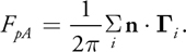
This equation, found in standard global illumination texts (such as Sillion and Puech 1994), computes the form factor from a polygonal source A to a point p with normal n. With each edge e _i of A, we associate a unit vector, _i . _i is formed by taking the cross product of a vector pointing along e _i with a vector pointing from p to e _i 's start vertex. For each edge of A, we dot _i with n, and sum. Figure 12-4 illustrates the approach.

Figure 12-4 Point-to-Polygon Form Factor

This equation assumes that the entire polygon is visible. For our application, we need to determine the visible portion of the polygon by clipping it to our shading point's plane of support. This is simply the plane passing through the point to be shaded facing in a direction equal to the shading normal. Not performing this clipping will over-estimate the true form factor and produce disturbing artifacts. Figure 12-5 shows the geometry of the clip.

Figure 12-5 Clipping a Triangle to a Visible Quadrilateral

Clipping a triangle by a plane results in one of three cases:

The entire triangle lies under the plane and is not visible.
The triangle lies partially under the plane and is partially visible. In this case, we clip the triangle to produce a quadrilateral.
The triangle lies completely above the plane and is completely visible.

Our clipping algorithm works by inspecting the triangle's three vertices with respect to the clipping plane. A point may lie above or under a plane, but for robustness issues, we also allow a point to lie on the plane. For three vertices with three possible configurations, there are 3³ = 27 possible configurations in all. Fortunately, the GeForce 8800's powerful branch performance quickly determines the configuration and tests only five branch conditions in the worst case.

Listing 12-2 shows our function that computes the visible portion of a triangle. The function accepts the clipping plane described by a point and normal, and the three vertices of the triangle to be clipped as input. It outputs the four vertices of the visible quad of the triangle. Note that a degenerate quad with two equal vertices may describe a fully visible triangle. Similarly, a degenerate quad with four equal vertices may describe an invisible triangle.

We begin by specifying an epsilon value that will control the robustness of the clip. Vertices that are closer to the plane than this value will be considered to lie on the plane. Next, we evaluate the plane equation for each vertex. This results in a signed distance from each vertex to the plane. Points above the plane have a positive distance; points below, a negative distance. Points that are too close to the plane have their distance clamped to zero.

Example 12-2. Finding the Visible Quadrilateral Portion of a Triangle

    void visibleQuad(float3 p,                  float3 n,                  float3 v0,                  float3 v1,                  float3 v2,              out float3 q0,              out float3 q1,              out float3 q2,              out float3 q3) {   const float epsilon = 1e-6;   float d = dot(n, p);   // Compute the signed distances from the vertices to the plane.    float sd[3]; sd[0] = dot(n, v0) – d;   if(abs(sd[0]) <= epsilon) sd[0] = 0.0;   sd[1] = dot(n, v1) – d;   if(abs(sd[1]) <= epsilon) sd[1] = 0.0;   sd[2] = dot(n, v2) – d;   if(abs(sd[2]) <= epsilon) sd[2] = 0.0;   // Determine case.    if(sd[0] > 0.0)   {     if(sd[1] > 0.0)     {       if(sd[2] < 0.0)       {         // v0, v1 above, v2 under         q0 = v0;         q1 = v1;         // Evaluate ray-plane equations:         q2 = v1 + (sd[1]/(sd[1] - sd[2])) * (v2 - v1);         q3 = v0 + (sd[0]/(sd[0] - sd[2])) * (v2 - v0);       }       else       {         // v0, v1, v2 all above         q0 = v0;         q1 = v1;         q2 = v2;         q3 = q3;       }     }   }   // Other cases similarly   . . .

We clip the triangle by inspecting the signs of these distances. When two signs match but the other does not, we must clip. In this case, two of the triangle's edges intersect the plane. The intersection points define two vertices of the visible quad. Depending on which edges intersect the plane, we evaluate two ray-plane intersection equations. With the visible portion of the triangle computed, we can compute its form factor with a straightforward implementation of the form factor equation applied to quadrilaterals.

12.4 Results

Next, we compare the results of our improved algorithm to those of the original. We chose two tests, the bunny and a car, to demonstrate the effectiveness of the new solution over a range of input. The bunny is a smooth, well-tessellated mesh with fairly equilateral triangles. In contrast, the car has heterogeneous detail with sharp angles and triangles with a wide range of aspect ratios. Figures 12-6 and 12-7 show the results.

Figure 12-6 Ambient Occlusion Comparison on the Bunny

Figure 12-7 Ambient Occlusion Comparison on the Car

You can see that the original per-vertex algorithm is well suited to the bunny due to its dense and regular tessellation. However, both disk-shaped and linear interpolation artifacts are apparent. The new algorithm removes these artifacts.

However, the original algorithm performs worse on the car. The sparse tessellation reveals linear interpolation artifacts on the per-vertex result. Applying the original shader at per-fragment rates smooths out this interpolation but adds both disk-shaped discontinuities and pinching near vertices. Our new algorithm is robust for both of these kinds of artifacts and produces a realistic result.

12.5 Performance

Here we include a short discussion of performance. In all experiments, we set epsilon, which controls traversal depth, to 8. First, we measured the performance of the initial iterative steps that shade the disks of the coarse occlusion hierarchy. Our implementation of this step is no different from the original algorithm and serves as a comparison. Next, we measured the performance of our new shader with and without triangle clipping and form factors. We used a deferred shading method to ensure that only visible fragments were shaded. Finally, we counted the number of total fragments shaded to measure the shading rate. Table 12-1 and Figure 12-8 show our performance measurements.

Table 12-1. Performance Results

Model	Size in Triangles	Total Fragments Shaded	Total Disks Shaded
Bunny	69,451	381,046	138,901
Car	29,304	395,613	58,607

Figure 12-8 Performance Results

We found the performance of shading disks in the hierarchy to be roughly comparable to shading fragments with the high-quality form factor computations. We observed that the disk shading rate tended to be much lower than per-fragment shading. We believe this is due to a smaller batch size than the total number of fragments to be shaded. Including the high-quality form factor computation in the shader requires extensive branching and results in a lower shading rate. However, this addition ensures a robust result.

12.6 Caveats

We continue with some notes on applying our algorithm in practice. First, as we previously mentioned, our smoothing solution may not completely eliminate all discontinuities. However, in all cases we have been able to make them arbitrarily faint by increasing the traversal depth. Additionally, because this algorithm can only approximate visibility, the results are often biased on the side of exaggerated shadows and may not match a reference computed by a ray tracer. To control the depth of occlusion, we introduce some tunable parameters that are useful in controlling error or achieving a desired artistic result.

12.6.1 Forcing Convergence

Recall that this method approximates visibility by applying the occlusion algorithm to disks iteratively over several passes. In our experiments, we have found that this algorithm tends not to converge to a unique solution on general scenes. In particular, architectural scenes with high occlusion usually oscillate between two solutions. To deal with this, we iteratively apply the original occlusion algorithm to compute disk-to-disk occlusion for a few passes as before. Then, we force convergence by setting each disk's occlusion to a weighted minimum of the last two results. Figure 12-9 presents the results achieved with this adjustment; Listing 12-3 shows the code.

Figure 12-9 The Benefits of Using a Weighted Minimum

Example 12-3. Forcing Convergence

    float o0 = texture2DRect(occlusion0, diskLocation).x; float o1 = texture2DRect(occlusion1, diskLocation).x; float m = min(o0, o1); float M = max(o0, o1); // weighted blend occlusion = minScale * m + maxScale * M;

Here, occlusion0 and occlusion1 contain the results of the last two iterations of the occlusion solution. We set the result to be a blend of the two. Because this algorithm overestimates occlusion in general, we bias the final result toward the smaller value. We have found 0.7 and 0.3 to be good values for minScale and maxScale, respectively.

12.6.2 Tunable Parameters

We have noted that our method in general tends to overestimate ambient occlusion. In fact, a completely enclosed environment produces a black scene! In general, ambient occlusion may not necessarily be exactly the quantity we are interested in computing. More generally, we might be interested in a function that resembles ambient occlusion for nearby shadow casters but falls off smoothly with distance. Such a function will produce deep contrast in local details but will not completely shadow a closed environment. We introduce two tunable parameters to control this effect.

Distance Attenuation

First, we allow the occlusion contribution of an element (whether it is a disk or a triangle) to be attenuated inversely proportional to the distance to it squared. Adjusting this parameter tends to brighten the overall result, as Figure 12-10 illustrates. Listing 12-4 shows the details.

Figure 12-10 Parameters' Effect on Result

Example 12-4. Attenuating Occlusion by Distance

    // Compute the occlusion contribution from an element contribution = solidAngle(. . .); // Attenuate by distance contribution /= (1.0 + distanceAttenuation * e2);

Triangle Attenuation

We also attenuate the occlusion contribution from triangles at the finest level of the hierarchy. Recall that we account for point-to-triangle visibility with two factors: we clip each triangle to a plane and we modulate the form factor by the triangle's occlusion. The combination of both of these factors can underestimate the true visibility, because the form factor of the clipped triangle is further dampened by modulation. We can compensate for this by raising the triangle's occlusion to a power before it is multiplied by its form factor and added to the sum. Low values for this parameter emphasize small features such as creases and cracks, which would otherwise be lost. High values lessen the influence of large, distant triangles that are probably not visible. In particular, you can see this parameter's influence on the stairs' shading in Figure 12-10. Listing 12-5 shows the details.

Example 12-5. Triangle Attenuation

    // Get the triangle's occlusion.    float elementOcclusion = . . . // Compute the point-to-triangle form factor. contribution = computeFormFactor(. . .); // Modulate by its occlusion raised to a power. contribution *= pow(elementOcclusion, triangleAttenuation);

12.7 Future Work

We have presented a robust, GPU-accelerated algorithm for computing high-quality ambient occlusion. By adaptively traversing the approximation of a shadow caster, we both quickly produce smooth soft shadows and reconstruct sharp local details.

We conclude by noting that this adaptive integration scheme is not limited to computing ambient occlusion. Bunnell 2005 showed how the same scheme could be used to compute indirect lighting. We also point out that subsurface scattering may be computed with the same hierarchical integration method. As shown in Figure 12-11, we can implement a multiple scattering technique (Jensen and Buhler 2002) in our framework simply by computing irradiance at each disk and then replacing calls to solidAngle() with multipleScattering(). Listing 12-6 shows the details.

Figure 12-11 Multiple Scattering Implemented via Hierarchical Integration

Example 12-6. Implementing Multiple Scattering

    float3 multipleScattering(float d2,                           float3 zr,     // Scattering parameters    float3 zv,     // defined in    float3 sig_tr) // Jensen and Buhler 2002 {   float3 r2  = float3(d2, d2, d2);   float3 dr1 = rsqrt(r2 + (zr * zr));   float3 dv1 = rsqrt(r2 + (zv * zv));   float3 C1  = zr * (sig_tr + dr1);   float3 C2  = zv * (sig_tr + dv1);   float3 dL  = C1 * exp(-sig_tr/dr1) * dr1 * dr1;          dL += C2 * exp(-sig_tr/dv1) * dv1 * dv1;   return dL; }

We include this effect alongside our ambient occlusion implementation on this book's accompanying DVD. Because many illumination effects may be defined as an integral over scene surfaces, we encourage the reader to generalize this technique to quickly generate other dazzling effects.

12.8 References

Bunnell, Michael. 2005. "Dynamic Ambient Occlusion and Indirect Lighting." In GPU Gems 2, edited by Matt Pharr, pp. 223–233. Addison-Wesley.

Jensen, Henrik Wann, and Juan Buhler. 2002. "A Rapid Hierarchical Rendering Technique for Translucent Materials." In ACM Transactions on Graphics (Proceedings of SIGGRAPH 2002) 21(3).

Sillion, François X., and Claude Puech. 1994. Radiosity and Global Illumination. Morgan Kaufmann.

Part II: Light and Shadows

Part III: Rendering

Part IV: Image Effects

Part V: Physics Simulation

Part VI: GPU Computing

Preface