
GPU Gems 3
GPU Gems 3 is now available for free online!
The CD content, including demos and content, is available on the web and for download.
You can also subscribe to our Developer News Feed to get notifications of new material on the site.
Chapter 10. Parallel-Split Shadow Maps on Programmable GPUs
Fan Zhang
The Chinese University of Hong Kong
Hanqiu Sun
The Chinese University of Hong Kong
Oskari Nyman
Helsinki University of Technology
Shadow mapping (Williams 1978) has been used extensively in 3D games and applications for producing shadowing effects. However, shadow mapping has inherent aliasing problems, so using standard shadow mapping is not enough to produce high-quality shadow rendering in complex and large-scale scenes. In this chapter we present an advanced shadow-mapping technique that produces antialiased and real-time shadows for large-scale environments. We also show the implementation details of our technique on modern programmable GPUs.
10.1 Introduction
The technique we present is called parallel-split shadow maps (PSSMs) (Zhang et al. 2007 and Zhang et al. 2006). In this technique the view frustum is split into multiple depth layers using clip planes parallel to the view plane, and an independent shadow map is rendered for each layer, as shown in Figure 10-1.
)
Figure 10-1 Parallel-Split Shadow Maps in
The split scheme is motivated by the observation that points at different distances from the viewer need different shadow-map sampling densities. By splitting the view frustum into parts, we allow each shadow map to sample a smaller area, so that the sampling frequency in texture space is increased. With a better matching of sampling frequencies in view space and texture space, shadow aliasing errors are significantly reduced.
In comparison with other popular shadow-mapping techniques, such as perspective shadow maps (PSMs) (Stamminger and Drettakis 2002), light-space perspective shadow maps (LiSPSMs) (Wimmer et al. 2004) and trapezoidal shadow maps (TSMs) (Martin and Tan 2004), PSSMs provide an intuitive way to discretely approximate the warped distribution of the shadow-map texels, but without mapping singularities and special treatments.
The idea of using multiple shadow maps was introduced in Tadamura et al. 2001. It was further studied in Lloyd et al. 2006 and implemented as cascaded shadow mapping in Futuremark's benchmark application 3DMark 2006.
The two major problems with all these algorithms, including our PSSMs, are the following:
- How do we determine the split positions?
- How do we alleviate the performance drop caused by multiple rendering passes when generating shadow maps and rendering the scene shadows?
These two problems are handled well in PSSMs. We use a fast and robust scene-independent split strategy to adapt the view-driven resolution requirement, and we show how to take advantage of DirectX 9-level and DirectX 10-level hardware to improve performance.
10.2 The Algorithm
In this chapter we use a directional light to illustrate the PSSMs technique for clarity, but the
implementation details are valid for point lights as well. The notation PSSM(m, res) denotes
the split scheme that splits the view frustum into m parts; res is the resolution for each
shadow map. Figure 10-2 shows the general
configuration for the split scheme with an overhead light, in which the view frustum V is split into
{Vi | 0
 i
m - 1} using clip planes at {Ci | 0
i
m} along the z axis. In particular, C 0 = n (near plane position)
and C m = f(far plane position).
i
m - 1} using clip planes at {Ci | 0
i
m} along the z axis. In particular, C 0 = n (near plane position)
and C m = f(far plane position).
)
Figure 10-2 The Configuration for the Split Scheme with an Overhead Light
We apply the split-scheme PSSM(m, res) in the following steps:
- Split the view frustum V into m parts {Vi } using split planes at {Ci }.
- Calculate the light's view-projection transformation matrix for each split part Vi .
- Generate PSSMs {Ti } with the resolution res for all split parts {Vi }.
- Synthesize shadows for the scene.
10.2.1 Step 1: Splitting the View Frustum
The main problem in step 1 is determining where the split planes are placed. Although users can adjust the split positions according to an application-specific requirement, our implementations use the practical split scheme proposed in Zhang et al. 2006.
Before we introduce this split scheme, we briefly review the aliasing problem in shadow mapping, which has been extensively discussed in Stamminger and Drettakis 2002, Wimmer et al. 2004, and Lloyd et al. 2006.
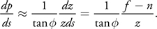
In Figure 10-3, the light beams passing through a
texel (with the size ds) fall on a surface of the object with the length dz in world space.
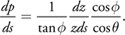
From the standard projection matrix in Direct3D, we know that the size of view beams dp (on the
normalized screen) projected from the surface is dy(z tan )-1, where
2 is the field-of-view of the view frustum. From the local view of the surface in
Figure 10-3, we get the approximation dy
 dz cos f/cos , where and stand for the angles between the surface
normal and vector to the screen, and the shadow-map plane, respectively.
dz cos f/cos , where and stand for the angles between the surface
normal and vector to the screen, and the shadow-map plane, respectively.
)
Figure 10-3 Shadow Map Aliasing
Shadow-Map Aliasing
The aliasing error for the small surface is then defined as
We usually decompose this aliasing representation dp/ds into two parts: perspective aliasing dz/zds and projection aliasing cos /cos (note that is a constant for a given view matrix). Shadow-map undersampling can occur when perspective aliasing or projection aliasing becomes large.
Projection aliasing depends on local geometry details, so the reduction of this kind of aliasing requires an expensive scene analysis at each frame. On the other hand, perspective aliasing comes from the perspective foreshortening effect and can be reduced by warping the shadow plane, using a perspective projection transformation. More important, perspective aliasing is scene independent, so the reduction of perspective aliasing doesn't require complicated scene analysis.
The practical split scheme is based on the analysis of perspective aliasing.
The Practical Split Scheme
In the practical split scheme, the split positions are determined by this equation:

where {
) } and {
} and {
) } are the split positions in the logarithmic split scheme and the uniform split scheme,
respectively. Theoretically, the logarithmic split scheme is designed to produce optimal distribution of
perspective aliasing over the whole depth range. On the other hand, the aliasing distribution in the uniform
split scheme is the same as in standard shadow maps.
Figure 10-4 visualizes the three split schemes in the
shadow-map space.
} are the split positions in the logarithmic split scheme and the uniform split scheme,
respectively. Theoretically, the logarithmic split scheme is designed to produce optimal distribution of
perspective aliasing over the whole depth range. On the other hand, the aliasing distribution in the uniform
split scheme is the same as in standard shadow maps.
Figure 10-4 visualizes the three split schemes in the
shadow-map space.
)
Figure 10-4 Visualization of the Practical Split Scheme in Shadow-Map Space
The theoretically optimal distribution of perspective aliasing makes dz/zds constant over the entire depth range. As shown in Wimmer et al. 2004, the following simple derivation gives the optimal shadow-map parameterization s(z):
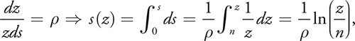
where is a constant. From s(f) = 1, we have = ln(f/n).
The only nonlinear transform supported by current hardware is the perspective-projection transformation
(s = A/z + B), so in order to approximate the previous logarithmic mapping
from z to s, the logarithmic split scheme discretizes it at several depth layers z =
as in the following equation:
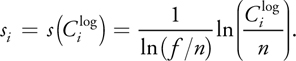
Because the logarithmic split scheme is designed to produce the theoretically even distribution of perspective aliasing, the resolution allocated for each split should be 1/m of the overall texture resolution. Substituting si = i/m into the preceding equation gives
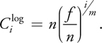
The main drawback of the logarithmic split scheme is that, in practice, the lengths of split parts near the viewer are too small, so few objects can be included in these split parts. Imagine the situation in the split-scheme PSSM(3)—that is, the view frustum is split into three parts. With f = 1000 and n = 1, the first split V 0 and second split V 1 occupy only 1 percent and 10 percent of the view distance. Oversampling usually occurs for parts near the viewer, and undersampling occurs for parts farther from the viewer. As a result, in practice, the logarithmic split scheme is hard to use directly.
The uniform split scheme simply places the split planes evenly along the view direction:
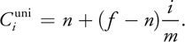
The aliasing distribution in the uniform split scheme is the same as that in standard shadow maps. Because s = (z- n)/(f - n) in standard shadow maps, by ignoring the projection aliasing, we have
This means the aliasing error in standard shadow maps increases hyperbolically as the object moves near the view plane. Like standard shadow mapping, the uniform split scheme results in undersampling for objects near the viewer and oversampling for distant objects.
Because the logarithmic and uniform split schemes can't produce appropriate sampling densities for the near and far depth layers simultaneously, the practical split scheme integrates logarithmic and uniform schemes to produce moderate sampling densities over the whole depth range. The weight adjusts the split positions according to practical requirements of the application. = 0.5 is the default setting in our current implementation. In Figure 10-4, the practical split scheme produces moderate sampling densities for the near and far split parts. An important note for Figure 10-4: the colorized sampling frequency in each split scheme is for schematic illustration only, not for precisely visualizing the aliasing distribution in theory. Readers interested in the (perspective) aliasing distributions in multiple depth layers can refer to Lloyd et al. 2006.
Preprocessing
Before splitting the view frustum, we might adjust the camera's near and far planes so that the view frustum contains the visible objects as tightly as possible. This will minimize the amount of empty space in the view frustum, increasing the available shadow-map resolution.
10.2.2 Step 2: Calculating Light's Transformation Matrices
As in standard shadow mapping, we need to know the light's view and projection matrices when generating the shadow map. As we split the light's frustum W into multiple subfrusta {Wi }, we will need to construct an independent projection matrix for each W i separately.
We present two methods to calculate these matrices:
- The scene-independent method simply bounds the light's frustum Wi to the split frustum
Vi , as seen in Figure 10-5.
Because information about the scene is not used, the usage of shadow-map resolution might not be optimal.
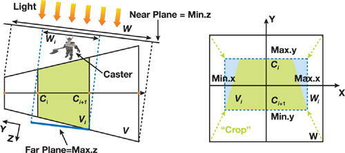
Figure 10-5 Calculation of the Light's Projection Matrix for the Split Part .
- The scene-dependent method increases the available texture resolution by focusing the light's frustum
Wi on the objects that potentially cast shadows to the split frustum
Vi , as seen later in
Figure 10-6.
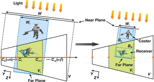
Figure 10-6 Comparing Projection Methods
)
)
Scene-Independent Projection
Before calculating the projection matrix for the subfrustum Wi , we must find the axisaligned bounding box (AABB) of the split frustum Vi with respect to the light's coordinates frame. The class BoundingBox is represented in Figure 10-5 using two vectors—a minimum vector and a maximum vector—to store the smallest and largest coordinates, respectively.
To simplify the computations, we determine the axis-aligned bounding box of the split frustum in the light's clip space, using the function CreateAABB(). Note that we set the bounding box's minimum z-value to 0 because we want the near plane position to remain unchanged. We want this position unchanged because we might have shadow casters between the near plane of the split's bounding box and the light's near plane. This case is illustrated by the "caster" object in Figure 10-5.
Afterward, we build a crop matrix to effectively "zoom in" the light's frustum Wi to the bounding box computed by CreateAABB(). The crop matrix is an off-center orthogonal projection matrix, computed as shown in Listing 10-1.
Example 10-1. Pseudocode for Constructing a Crop Matrix from Clip-Space Bounding Values
// Build a matrix for cropping light's projection
// Given vectors are in light's clip space Matrix
Light::CalculateCropMatrix(Frustum splitFrustum)
{
  Matrix lightViewProjMatrix = viewMatrix * projMatrix;
  // Find boundaries in light's clip space
  BoundingBox cropBB = CreateAABB(splitFrustum.AABB, lightViewProjMatrix);
  // Use default near-plane value
  cropBB.min.z = 0.0f;
  // Create the crop matrix
  float scaleX, scaleY, scaleZ;
  float offsetX, offsetY, offsetZ;
  scaleX = 2.0f / (cropBB.max.x - cropBB.min.x);
  scaleY = 2.0f / (cropBB.max.y - cropBB.min.y);
  offsetX = -0.5f * (cropBB.max.x + cropBB.min.x) * scaleX;
  offsetY = -0.5f * (cropBB.max.y + cropBB.min.y) * scaleY;
  scaleZ = 1.0f / (cropBB.max.z - cropBB.min.z);
  offsetZ = -cropBB.min.z * scaleZ;
  return Matrix(scaleX, 0.0f, 0.0f, 0.0f, 0.0f, scaleY, 0.0f, 0.0f, 0.0f, 0.0f,
                scaleZ, 0.0f, offsetX, offsetY, offsetZ, 1.0f);
}
Finally, we use the light's view-projection transformation lightViewMatrix * lightProjMatrix * cropMatrix when generating the shadow map texture Ti .
Note that instead of computing a crop matrix in the light's clip space, we can calculate the split-specific projection matrix in other spaces, such as the light's view space. However, because both point and directional lights are converted into directional lights in the light's clip space, our method works the same way for directional and point lights. Furthermore, calculating the bounding box in the light's clip space is more intuitive.
Scene-Dependent Projection
Although using a scene-independent projection works well in most cases, we can further optimize the usage of the texture resolution by taking the scene geometries into account.
As we can see in Figure 10-6, a scene-independent Wi may contain a large amount of empty space. Each Wi only needs to contain the objects potentially casting shadows into Vi , termed shadow casters, exemplified by BC . Because the invisible parts of objects don't need to be rendered into the final image, we separately store the shadow-related objects inside (or partially inside) Vi as shadow receivers, exemplified by BR . When synthesizing the shadowed image of the whole scene, we render only shadow receivers to improve rendering performance. Note that objects that never cast shadows (such as the terrain) should be included in receivers only.
In the scene-dependent method, the near plane of Wi is moved to bound either Vi or any shadow caster, and the far plane of Wi is moved to touch either Vi or any shadow receiver. The optimized near and far planes improve the precision of discrete depth quantization. Furthermore, because only shadow receivers need to do depth comparison during shadow determination, we adjust the x- and y-boundaries of Wi to bound Vi or any shadow receiver. The pseudocode for the scene-dependent method is shown in Listing 10-2. Pay special attention to how the depth boundaries (min.z and max.z) are chosen.
The final light's view-projection transformation matrix for the current split is still lightViewMatrix * lightProjMatrix * cropMatrix.
Example 10-2. Pseudocode for Computing Scene-Dependent Bounds
Matrix Light::CalculateCropMatrix(ObjectList casters, ObjectList receivers,
                                  Frustum frustum)
{
  // Bounding boxes
  BoundingBox receiverBB, casterBB, splitBB;
  Matrix lightViewProjMatrix = viewMatrix * projMatrix;
  // Merge all bounding boxes of casters into a bigger "casterBB".
  for (int i = 0; i < casters.size(); i++)
  {
    BoundingBox bb = CreateAABB(casters[i]->AABB, lightViewProjMatrix);
    casterBB.Union(bb);
  }
  // Merge all bounding boxes of receivers into a bigger "receiverBB".
  for (int i = 0; i < receivers.size(); i++)
  {
    bb = CreateAABB(receivers[i]->AABB, lightViewProjMatrix);
    receiverBB.Union(bb);
  }
  // Find the bounding box of the current split
  // in the light's clip space.
  splitBB = CreateAABB(splitFrustum.AABB, lightViewProjMatrix);
  // Scene-dependent bounding volume
  BoundingBox cropBB;
  cropBB.min.x = Max(Max(casterBB.min.x, receiverBB.min.x), splitBB.min.x);
  cropBB.max.x = Min(Min(casterBB.max.x, receiverBB.max.x), splitBB.max.x);
  cropBB.min.y = Max(Max(casterBB.min.y, receiverBB.min.y), splitBB.min.y);
  cropBB.max.y = Min(Min(casterBB.max.y, receiverBB.max.y), splitBB.max.y);
  cropBB.min.z = Min(casterBB.min.z, splitBB.min.z);
  cropBB.max.z = Min(receiverBB.max.z, splitBB.max.z);
  // Create the crop matrix.
  float scaleX, scaleY, scaleZ;
  float offsetX, offsetY, offsetZ;
  scaleX = 2.0f / (cropBB.max.x - cropBB.min.x);
  scaleY = 2.0f / (cropBB.max.y - cropBB.min.y);
  offsetX = -0.5f * (cropBB.max.x + cropBB.min.x) * scaleX;
  offsetY = -0.5f * (cropBB.max.y + cropBB.min.y) * scaleY;
  scaleZ = 1.0f / (cropBB.max.z – cropBB.min.z);
  offsetZ = -cropBB.min.z * scaleZ;
  return Matrix(scaleX, 0.0f, 0.0f, 0.0f, 0.0f, scaleY, 0.0f, 0.0f, 0.0f, 0.0f,
                scaleZ, 0.0f, offsetX, offsetY, offsetZ, 1.0f);
}
10.2.3 Steps 3 and 4: Generating PSSMs and Synthesizing Shadows
Steps 3 and 4 can be implemented differently, depending on your system hardware. Because we use multiple shadow maps in PSSMs, extra rendering passes may be needed when we generate shadow maps and synthesize shadows.
To reduce this burden on rendering performance, we could use a hardware-specific approach. In the next section we present three hardware-specific methods for generating PSSMs and synthesizing shadows:
- The multipass method (without hardware acceleration): This method doesn't use hardware acceleration; multiple rendering passes are required for generating shadow maps (step 3) and for synthesizing shadows (step 4).
- Partially accelerated on DirectX 9-level hardware (for example, Windows XP and an NVIDIA GeForce 6800 GPU): In this method, we remove extra rendering passes for synthesizing scene shadows.
- Fully accelerated on DirectX 10-level hardware (for example, Windows Vista and a GeForce 8800 GPU): Here we alleviate the burden of extra rendering passes for generating shadow maps. To achieve this goal, we describe two different approaches: geometry shader cloning and instancing.
In all three methods, the implementations for splitting the view frustum and calculating the light's transformation matrices are the same as described earlier.
10.3 Hardware-Specific Implementations
To make it easier to understand our three hardware-specific implementations, we visualize the rendering pipelines of different implementations, as in Figure 10-7.
)
Figure 10-7 Visualization of Rendering Pipelines
10.3.1 The Multipass Method
In the first implementation of PSSMs, we simply render each shadow map, with shadows in each split part, sequentially.
Generating Shadow Maps
Once we have the light's view-projection transformation matrix lightViewMatrix * lightProjMatrix * cropMatrix for the current split part, we can render the associated shadow-map texture. The procedure is the same as for standard shadow mapping: we render all shadow casters to the depth buffer. Our implementation uses a 32-bit floating-point (R32F) texture format.
In our multipass implementation, instead of storing PSSMs in several independent shadow-map textures, we reuse a single shadow-map texture in each rendering pass, as shown in Listing 10-3.
Example 10-3. Pseudocode for the Rendering Pipeline of the Multipass Method
for (int i = 0; i < numSplits; i++)
{
  // Compute frustum of current split part.
  splitFrustum = camera->CalculateFrustum(splitPos[i], splitPos[i + 1]);
  casters = light->FindCasters(splitFrustum);
  // Compute light's transformation matrix for current split part.
  cropMatrix = light->CalculateCropMatrix(receivers, casters, splitFrustum);
  splitViewProjMatrix = light->viewMatrix * light->projMatrix * cropMatrix;
  // Texture matrix for current split part
  textureMatrix = splitViewProjMatrix * texScaleBiasMatrix;
  // Render current shadow map.
  ActivateShadowMap();
  RenderObjects(casters, splitViewProjMatrix);
  DeactivateShadowMap();
  // Render shadows for current split part.
  SetDepthRange(splitPos[i], splitPos[i + 1]);
  SetShaderParam(textureMatrix);
  RenderObjects(receivers, camera->viewMatrix * camera->projMatrix);
}
Synthesizing Shadows
With PSSMs generated in the preceding step, shadows can now be synthesized into the scene. In the multipass method, we need to synthesize the shadows immediately after rendering the shadow map.
For optimal performance, we should render the splits from front to back. However, some special considerations are needed. We need to adjust the camera's near and far planes to the respective split positions to provide clipping, because the objects in one split may also overlap other splits. However, as we modify the near and far planes, we are also changing the range of values written to the depth buffer. This would make the depth tests function incorrectly, but we can avoid this problem by using a different depth range in the viewport. Simply convert the split-plane positions from view space to clip space and use them as the new depth minimum and maximum.
After this we can render the shadow receivers of the scene while sampling the shadow map in the standard manner. This means that implementing the multipass method doesn't require the use of shaders. Figure 10-8 compares SSM(2Kx2K) and multipass PSSM(3; 1Kx1K). However, as the method's name implies, multiple rendering passes will always be performed for both generating shadow maps and rendering scene shadows.
)
Figure 10-8 Comparison of SSM and Multipass PSSM
10.3.2 DirectX 9-Level Acceleration
When implementing the simple multipass method as presented, we need to use multiple rendering passes to synthesize shadows in the scene. However, with programmable GPUs, we can perform this step in a single rendering pass.
We can create a pixel shader to find and sample the correct shadow map for each fragment. The operation for determining which split a fragment is contained in is simple because the split planes are parallel to the view plane. We can simply use the depth value—or, as in our implementation, use the view space z coordinate of a fragment—to determine the correct shadow map.
The Setup
Because we render the scene shadows in a single pass, we need to have access to all the shadow maps simultaneously. Unlike our previous implementation, this method requires that shadow maps be stored separately, so we create an independent texture for each shadow map.
Note that the number of texture samplers supported by the hardware will limit the number of shadow maps we can use. We could, alternatively, pack multiple shadow maps in a single texture; however, most DirectX 9-level hardware supports eight texture samplers, which should be more than enough.
Also note that we need to use the "border color" texture address mode, because sometimes shadow maps are sampled outside the texture-coordinate range. This could occur when we use a scene-dependent projection, because the light's subfrustum Wi does not necessarily cover all the receivers.
Synthesizing Shadows
When we render the scene shadows, we use a custom vertex and pixel shader, as shown in Listing 10-4. In the vertex shader, we transform each vertex as usual. However, we also calculate (1) the view-space position of the vertex, because we will use it for determining the shadow maps associated with fragments; and (2) the position of the vertex in the texture space of each shadow map. We determine the position of the vertex by multiplying the vertex with a textureMatrix. It is the same approach we use for standard shadow mapping, only now we use it for all shadow maps. We output all the transformed coordinates into texture-coordinate registers for the pixel shader to use.
In the pixel shader, we loop through all splits and test whether the view-space distance of the fragment is less than the end position of the split. After determining the split index, we sample the associated shadow map with the associated texture coordinates and perform a standard shadow-map depth test.
Example 10-4. Vertex and Pixel Shaders for Synthesizing Shadows in DirectX 9
sampler2D shadowMapSampler[numSplits];
void VS_RenderShadows(in float4 pos : POSITION, // Object-space coordinates
                        out float4 posOut : POSITION, // Clip-space coordinates
                        out float4 texCoord[numSplits + 1] : TEXCOORD) // Texture coordinates
{
  // Calculate world position.
  float4 posWorld = mul(pos, worldMatrix);
  // Transform vertex.
  posOut = mul(posWorld, viewProjMatrix);
  // Store view-space position in the first texture
  // coordinate register.
  texCoord[0] = mul(posWorld, viewMatrix);
  // Store shadow-map coordinates in the remaining
  // texture coordinate registers.
  for (int i = 0; i < numSplits; i++)
  {
    texCoord[i + 1] = mul(posWorld, textureMatrix[i]);
  }
}
float4 PS_RenderShadows(float4 texCoord[numSplits + 1] : TEXCOORD) : COLOR
{
  float light = 1.0f;
  // Fetch view-space distance from first texture coordinate register.
  float distance = texCoord[0].z;
  for (int i = 0; i < numSplits; i++)
  {
    if (distance < splitPlane[i])
    {
      float depth = texCoord[i + 1].z / texCoord[i + 1].w;
      float depthSM = tex2Dproj(shadowMapSampler[i], texCoord[i + 1]);
      // Standard depth comparison
      light = (depth < depthSM) ? 1.0f : 0.0f;
      break;
    }
  }
  return light;
}
Performance
We implemented this partially accelerated method in both DirectX 9 and OpenGL. In DirectX 9, we implemented percentage-closer filtering (PCF) (Reeves et al. 1987) in the pixel shader (approximately 25 instructions), and in OpenGL we used hardware-accelerated PCF (one instruction). We compared the performance to the multipass method when we increased the number of objects in the scene. In all tests, the number of splits was four.
From the results shown in Figure 10-9, we can see that the DirectX 9-level acceleration increases performance. But when PCF is implemented in the pixel shader, the shaders become more complex. This increase in the shader complexity causes performance to decrease, but this becomes less significant as the scene complexity increases.
)
Figure 10-9 Performance Results with GeForce 6800 Ultra () and GeForce 8800 GTS ()
10.3.3 DirectX 10-Level Acceleration
Although rendering scene shadows is accelerated on DirectX 9-level hardware, multiple rendering passes are still required for generating PSSMs. In other words, DirectX 9 provides us a partial acceleration of PSSMs. On the other hand, we can accelerate both generating PSSMs and rendering scene shadows on DirectX 10-level hardware.
Features in Direct3D 10
The Direct3D 10 pipeline introduces the geometry shader (GS) as a new shader stage between vertex and pixel shaders. Geometry shaders are executed once for each primitive, taking the vertices of the primitive as input and outputting a number of new primitives. They also provide access to primitive adjacency information and have an instruction set similar to that of vertex shaders (including support for texture sampling).
Another new feature in Direct3D 10 is the render target array, which is similar to Direct3D 9's multiple render targets (MRTs). But while MRTs only enable separate pixel shader output for each render target, the render target arrays (with the help of geometry shaders) can output entirely different geometries to each render target. This is done in the GS output, where we can specify a render target index for each primitive separately.
These features enable us to dynamically "clone" the geometry into different render targets with different transformations. We can now improve the performance of generating PSSMs because each shadow caster needs to be submitted only once.
The Setup
First we need to create a texture array for the shadow maps. As shown in Listing 10-5, we use a 32-bit floating-point texel format as usual, but we define it as "typeless" because it will need to work both as a depth buffer and as a texture. The ArraySize parameter is set to the number of splits, so we have one texture for each. Also, we must set the BindFlags to allow us to bind the texture array to both a depth-stencil view and a shader resource view.
Resource views, another new feature in Direct3D 10, allow a single resource to be interpreted in different ways. In our case, we need to access the texture array both as a renderable depth-stencil surface and as a shader-accessible texture, so we must create views for both.
As shown in Listing 10-6, creating the shader resource view is simple. We set the view dimension to a texture 2D array and set the texel format to a single-channel floating-point color. Otherwise, we use the same settings as when we create the texture array.
The depth-stencil view is created in a similar manner, but the texel format must be set to a depth-buffer-compatible format, as shown in Listing 10-7.
Now we have an array of shadow maps that we can set as depth-stencil targets and bind as sampleable textures. Note that we don't need to create a render target, because we are interested in rendering only depth values, not color information.
We still have to create the needed shaders, which will be explained in the next two sub-sections.
Example 10-5. Creating a Texture Array
D3D10_TEXTURE2D_DESC DescTex = {};
DescTex.Width = shadowMapSize;
DescTex.Height = shadowMapSize;
DescTex.ArraySize = numSplits;
DescTex.Format = DXGI_FORMAT_R32_TYPELESS;
DescTex.Usage = D3D10_USAGE_DEFAULT;
DescTex.BindFlags = D3D10_BIND_DEPTH_STENCIL | D3D10_BIND_SHADER_RESOURCE;
DescTex.MipLevels = 1;
DescTex.SampleDesc.Count = 1;
device->CreateTexture2D(...)
Example 10-6. Creating a Shader Resource View
D3D10_SHADER_RESOURCE_VIEW_DESC DescSRV = {};
DescSRV.Format = DXGI_FORMAT_R32_FLOAT;
DescSRV.ViewDimension = D3D10_SRV_DIMENSION_TEXTURE2DARRAY;
DescSRV.Texture2DArray.ArraySize = numSplits;
DescSRV.Texture2DArray.MipLevels = 1;
device->CreateShaderResourceView(...)
Example 10-7. Creating a Depth-Stencil Resource View
D3D10_DEPTH_STENCIL_VIEW_DESC DescDSV = {};
DescDSV.Format = DXGI_FORMAT_D32_FLOAT;
DescDSV.ViewDimension = D3D10_DSV_DIMENSION_TEXTURE2DARRAY;
DescDSV.Texture2DArray.ArraySize = numSplits;
device->CreateDepthStencilView(...);
Generating Shadow Maps
The rendering pipeline looks similar to the DirectX 9 version. The major difference is that we render shadow maps only once. Also, we now need to store the crop matrices of each split into an array, because we will need them all in the shaders.
More important, after finding the potential shadow casters for a split, we need each caster to keep track of two variables: firstSplit and lastSplit. These variables determine the range of the split indices into which the shadow caster needs to be rendered, as shown in Figure 10-10. Note that we need to store only the first and last indices, because a continuous bounding shape will always overlap a continuous range of split parts.
)
Figure 10-10 The Shadow Caster Straddles the Split Parts from to
As we begin rendering the shadow maps, we need to set a new viewport and change the render targets. This is shown in Listing 10-8, where the variable pDSV points to the previously created depth-stencil view. Because we will only render depth information, we must set the number of render targets to 0 and the render target pointer to NULL.
Example 10-8. Activating Shadow-Map Rendering
D3D10_VIEWPORT vp;
vp.Width = shadowMapSize;
vp.Height = shadowMapSize;
vp.MinDepth = 0;
vp.MaxDepth = 1;
vp.TopLeftX = 0;
vp.TopLeftY = 0;
device->RSSetViewports(1, &vp);
device->OMSetRenderTargets(0, NULL, pDSV);
Then we draw each shadow caster once, but in a special rendering loop. In this loop, we must update the shader constants firstSplit and lastSplit with corresponding values from the shadow caster. Because these variables are "perinstance" data, they should be handled like, for example, an object's world matrix.
In the following, we present two different approaches for dynamically cloning the geometry for different splits.
Using Geometry Shader Cloning
In this first method, we use the geometry shader to clone submitted triangles into different render targets. This technique is similar to the single-pass cube map technique presented in the Microsoft DirectX SDK. We first explain the details here, and then we discuss the performance advantages.
With this technique, the vertex shader simply transforms each vertex with the world matrix, the light's view matrix, and the light's projection matrix. This transformation is common for all shadow casters, regardless of which shadow maps they must be rendered into. The split-specific transformations will be applied in the geometry shader instead, as visualized in Figure 10-11.
)
Figure 10-11 The GPU Rendering Pipeline in the Geometry Shader Cloning Method
In other words, we now use the geometry shader to clone triangles into the split-specific render targets and then transform these triangles with the corresponding crop matrices as well.
The geometry shader code is shown in Listing 10-9, where we loop through each split to be rendered—that is, from firstSplit to lastSplit. Inside this loop, we transform each vertex with the split's corresponding crop matrix. We also set a render target index, and then finally we output the transformed vertices as a new triangle. Note that the render target index is in fact specified per vertex, but only the value in the leading (first) vertex is relevant.
Example 10-9. Geometry Shader Code for Rendering Shadow Maps
// Geometry shader output structure
   struct GS_OUT
{
  float4 pos : SV_POSITION;
  uint RTIndex : SV_RenderTargetArrayIndex;
};
// Geometry shader
[maxvertexcount(NUMSPLITS * 3)]
void GS_RenderShadowMap(triangle VS_OUT In[3],
                        inout TriangleStream<GS_OUT> triStream)
{
  // For each split to render
   for(int split = firstSplit; split <= lastSplit; split++)
  {
    GS_OUT Out;
    // Set render target index.
    Out.RTIndex = split;
    // For each vertex of triangle
   for(int vertex = 0; vertex < 3; vertex++)
    {
      // Transform vertex with split-specific crop matrix.
      Out.pos = mul(In[vertex].pos, cropMatrix[split]);
      // Append vertex to stream
      triStream.Append(Out);
    }
    // Mark end of triangle
    triStream.RestartStrip();
  }
}
A pixel shader is not needed at this stage because we aren't interested in drawing color information. So, it can simply be set to NULL.
For the sake of clarity, the implementation we presented uses separate transformations for all matrices. By premultiplying view/projection/crop matrices together, we can implement the split-scheme PSSM(m) using this method such that the number of transformations is (1 + m) per vertex. That is, every vertex is transformed with the world matrix (one time) and then with the view/projection/crop matrices (m times). Standard shadow-map rendering with a similar setup would use (m + m) transformations. However, if we premultiply the world matrices as well, the number of transformations is the same (m) for both methods. The advantage of the geometry shader cloning method is that it reduces the API overhead—the overhead of extra draw calls, render target switches, and so on is removed because we submit each shadow caster only once.
Using Instancing
The second approach for generating shadow maps is possible with the improved instancing support in Direct3D 10. Vertex shaders can now acquire the index of an instance being rendered through the semantic SV_InstanceID.
This means we can use instancing to clone our geometry for each split, and determine the split index from the instance index. We can then perform the crop matrix transformation in the vertex shader, so that the only task left for the geometry shader is setting the render target index, as shown in Listing 10-10 and visualized in Figure 10-12.
)
Figure 10-12 The GPU Rendering Pipeline in the Instancing Method
To render with instancing, we need to call the function DrawIndexedInstanced() with the number of instances set to lastSplit - firstSplit + 1. This is the only change needed on the CPU side; it is not necessary to set up any extra vertex streams.
Example 10-10. Vertex and Geometry Shaders for Generating Shadow Maps with Instancing
   struct VS_IN
{
  float4 pos : POSITION;
  uint instance : SV_InstanceID;
};
struct VS_OUT
{
  float4 pos : POSITION;
  uint split : TEXTURE0;
};
VS_OUT VS_RenderShadowMap(VS_IN In)
{
  VS_OUT Out;
  // Transform with world/view/projection.
  Out.pos = mul(In.pos, ...);
  // Determine split index from instance ID.
  Out.split = firstSplit + In.instance;
  // Transform with split-specific crop matrix.
  Out.pos = mul(Out.pos, cropMatrix[Out.split]);
  return Out;
}
[maxvertexcount(3)]
void GS_RenderShadowMap(triangle VS_OUT In[3],
                        inout TriangleStream<GS_OUT> triStream)
{
  GS_OUT Out;
  // Set render target index.
  Out.RTIndex = In[0].split;
  // Pass triangle through.
  Out.pos = In[0].pos;
  triStream.Append(Out);
  Out.pos = In[1].pos;
  triStream.Append(Out);
  Out.pos = In[2].pos;
  triStream.Append(Out);
  triStream.RestartStrip();
}
Using this method, we again remove the extra API overhead. However, the number of transformations is the same as with standard shadow-map rendering. Still, the instancing method may be faster than using geometry shader cloning because expanding large amounts of data with the geometry shader may be expensive.
We can also use the cloning and instancing methods together, so that both are used to generate geometry for a portion of the splits. For example, in the split-scheme PSSM(4), instancing could be used for two splits and geometry shader cloning for another two splits.
Synthesizing Shadows
The process of rendering shadows is nearly the same as in DirectX 9. The main difference is in the sampling of the texture array. To do things the traditional way, we can use the function SampleLevel() to sample from a given texture of the array.
Using this function is straightforward, but note that the second parameter is a float3, where the first two floats are for the UV coordinates and the third float is for the texture index. The mipmap level is defined in the function's third parameter.
After sampling the correct texture with this function, we would perform the depth comparison as usual. However, this is not the optimal method, especially if we wish to use PCF. We present a better approach next, which uses cube maps.
Using Cube Maps
HLSL 4 introduces a new function called SampleCmpLevelZero(), which performs sampling and comparison simultaneously. It can also be used with a linear comparison filter to get PCF, which means the function will take four samples, compare each separately, and then bilinearly filter the results.
Unfortunately, SampleCmpLevelZero() cannot currently be used with Texture2DArrays. It can, however, be used with TextureCubes. TextureCubes are normally used for cube maps, but they are essentially a texture array with six textures, one for each face of the cube.
This means we can use a TextureCube for up to six splits. Using a TextureCube requires only a few changes in the setup, as shown in Listing 10-11. Rendering shadow maps works the same way as before.
Sampling is slightly complicated by the fact that a cube map is not accessed with standard texture coordinates, but instead with a vector pointing to a face of the cube. This cube is a unit cube, and it is centered in the origin. The faces are ordered so that from array index 0 to 5, the faces are located at +x, -x, +y, -y, +z, and -z, respectively. From this we can determine the correct direction vector for accessing each face, as shown in Listing 10-12.
However, the approach shown in Listing 10-12 is not necessary, because we can separate the different cases into three lookup arrays, as shown in Listing 10-13, which slightly increases the pixel shader's performance.
Another issue is that border color addressing mode cannot be used, because the borders are simply mapped onto another face of the cube map. However, we can simulate the border color addressing mode by avoiding sampling altogether if the coordinates are outside the valid range of texture coordinates. This is also shown in Listing 10-13.
In our tests, using SampleCmpLevelZero() with a TextureCube slightly improved our performance compared to using a Texture2DArray with four-tap PCF implemented in the pixel shader (approximately 25 instructions). However, with a TextureCube, six textures will always be allocated even if fewer are needed, often resulting in wasted memory.
Example 10-11. Changes Needed for Creating a TextureCube
// When creating the texture array
DescTex.ArraySize = 6;
DescTex.MiscFlags = D3D10_RESOURCE_MISC_TEXTURECUBE;
. . .
// When creating the shader resource view
DescSRV.ViewDimension = D3D10_SRV_DIMENSION_TEXTURECUBE;
DescSRV.TextureCube.MipLevels = 1;
Example 10-12. Choosing Faces from a TextureCube
float3 cubeCoord;
if (split == 0)
  cubeCoord = float3(0.5, 0.5 - pos.y, 0.5 - pos.x);
else if (split == 1)
  cubeCoord = float3(-0.5, 0.5 - pos.y, pos.x - 0.5);
else if (split == 2)
  cubeCoord = float3(pos.x - 0.5, 0.5, pos.y - 0.5);
else if (split == 3)
  cubeCoord = float3(pos.x - 0.5, -0.5, 0.5 - pos.y);
else if (split == 4)
  cubeCoord = float3(pos.x - 0.5, 0.5 - pos.y, 0.5);
else if (split == 5)
  cubeCoord = float3(0.5 - pos.x, 0.5 - pos.y, -0.5);
Example 10-13. Pixel Shader Code for Synthesizing Shadows with a TextureCube
   static const float3 offset[6] = {
  float3(0.5, 0.5, 0.5), float3(-0.5, 0.5, -0.5),
  float3(-0.5, 0.5, -0.5), float3(-0.5, -0.5, 0.5),
  float3(-0.5, 0.5, 0.5), float3(0.5, 0.5, -0.5)};
static const float3 mulX[6] = {
  float3(0, 0, -1), float3(0, 0, 1), float3(1, 0, 0),
  float3(1, 0, 0), float3(1, 0, 0), float3(-1, 0, 0)};
static const float3 mulY[6] = {
  float3(0, -1, 0), float3(0, -1, 0), float3(0, 0, 1),
  float3(0, 0, -1), float3(0, -1, 0), float3(0, -1, 0)};
SamplerComparisonState shadowMapSampler
{
  ComparisonFunc = Less;
  Filter = COMPARISON_MIN_MAG_LINEAR_MIP_POINT;
};
float4 PS_RenderShadows(PS_INPUT In) : SV_Target
{
  float light = 1.0f;
  for(int split = 0; split < numSplits; split++)
  {
    if(In.distance > splitEnd[split])
    {
      float4 texpos = In.texturePos[split];
      texpos.xyz /= texpos.w;
      // Cube map vector lookup
   float3 cubeCoord = offset[split] +
                          mulX[split] * texpos.x +
                          mulY[split] * texpos.y;
      // Don't sample outside the border.
   if(min(pos.x, pos.y) > 0 && max(pos.x, pos.y) < 1)
      {
        light = shadowMapCube.SampleCmpLevelZero(shadowMapSampler,
                                                 cubeCoord, texpos.z);
      }
      break;
    }
  }
  return light;
}
10.4 Further Optimizations
To improve the shadow quality with PSSMs, use the following optimizations:
- Filtering Techniques. Percentage-closer filtering (PCF) helps antialiasing in shadow mapping by performing multiple depth tests for each pixel, which makes the shadow boundaries look considerably smoother. Variance shadow maps (VSMs) (Donnelly and Lauritzen 2006) treat shadow map texels as a distribution of depths and represent this distribution in a way that can be linearly filtered. Chebyshev's inequality is used to approximate the occlusion over an arbitrary filter region.
- Packing of Textures. Instead of storing PSSMs into multiple textures in hardware-accelerated implementations, users may pack them into a single texture. This is a possible solution when few texture samplers are available. In DirectX 10, texture arrays can be utilized instead.
- Warping Algorithms. An interesting application of the split scheme is applying warping algorithms (for example, PSMs, LiSPSMs, and TSMs) separately in split parts.
- Varying Texture Resolution. All shadow maps in our current implementation of PSSMs have the same resolution. To reduce the required consumption of textures, users can adjust the size of each shadow map at different split layers.
- Linearized Depth Distribution (Brabec et al. 2002). Using a linear depth metric instead of standard projected z increases the precision of discrete depth quantization for point lights.
10.5 Results
The screen shots in Figures 10-13 through 10-16 from Dawnspire: Prelude—displayed throughout the remainder of the chapter—were rendered using the PSSM(3; 1Kx1K) scheme (multipass method) at an image size of 1280x1024. The performance is measured on a PC configured with an AMD Athlon64 X2 3800 CPU, 1 GB DDR RAM, and a GeForce 7800 GTX GPU. The number of visible triangles processed in these figures ranges from 165 K to 319 K. In our experiments, both PSSM(3) and PSSM(4) achieve a good trade-off between the performance and visual qualities (more than 31 frames/sec and 27 frames/sec in the two schemes, respectively).
)
Figure 10-13 Screen Shot from
)
Figure 10-14 From
)
Figure 10-15 From
)
Figure 10-16 From
In many applications, especially for complex and large-scale scenes, rendering high-quality shadows is crucial for the users' perception of realism. Even without hardware acceleration, it is worth the cost of multipass rendering to dramatically improve shadow quality.
10.6 Conclusion
The basic idea of parallel-split shadow maps is intuitive and simple to implement, as with our multipass method. We can quickly determine the split positions using the practical split scheme without complicated scene analysis. However, without using hardware acceleration, the performance drop caused by multiple rendering passes prevents this technique from being extensively used in mass-market applications.
In this chapter, we present two hardware-accelerated methods: partially accelerated implementation on DirectX 9-level GPUs and fully accelerated implementation on DirectX 10-level GPUs. The extra rendering passes required for synthesizing shadows are avoided in the partially accelerated implementation. In the DirectX 10 rendering pipeline, our fully accelerated implementation reduces the cost of extra rendering passes for rendering both shadow maps and scene shadows.
There are many other ways to improve performance and shadow quality in our PSSMs technique, but one thing is certain: With the rapid evolution of GPUs, PSSMs are a promising approach for high-quality shadow rendering.
Demos with full source code can be found on the book's accompanying DVD. All three implementation methods presented in this chapter are included.
10.7 References
Brabec, Stefan, Thomas Annen, and Hans-Peter Seidel. 2002. "Practical Shadow Mapping." Journal of Graphical Tools 7(4), pp. 9–18.
Donnelly, William, and Andrew Lauritzen. 2006. "Variance Shadow Maps." In Proceedings of the Symposium on Interactive 3D Graphics and Games 2006, pp. 161–165.
Lloyd, Brandon, David Tuft, Sung-Eui Yoon, and Dinesh Manocha. 2006. "Warping and Partitioning for Low Error Shadow Maps." In Proceedings of the Eurographics Symposium on Rendering 2006, pp. 215–226.
Martin, Tobias, and Tiow-Seng Tan. 2004. "Anti-aliasing and Continuity with Trapezoidal Shadow Maps." In Proceedings of the Eurographics Symposium on Rendering 2004, pp. 153–160.
Reeves, William, David Salesin, and Robert Cook. 1987. "Rendering Antialiased Shadows with Depth Maps." In Computer Graphics (Proceedings of SIGGRAPH 1987) 21(3), pp. 283–291.
Stamminger, Marc, and George Drettakis. 2002. "Perspective Shadow Maps." In ACM Transactions on Graphics (Proceedings of SIGGRAPH 2002) 21(3), pp. 557–562.
Tadamura, Katsumi, Xueying Qin, Guofang Jiao, and Eihachiro Nakamae. 2001. "Rendering Optimal Solar Shadows with Plural Sunlight Depth Buffers." The Visual Computer 17(2), pp. 76–90.
Williams, Lance. 1978. "Casting Curved Shadows on Curved Surfaces." In Computer Graphics (Proceedings of SIGGRAPH 1978) 12(3), pp. 270–274.
Wimmer, Michael, Daniel Scherzer, and Werner Purgathofer. 2004. "Light Space Perspective Shadow Maps." In Proceedings of the Eurographics Symposium on Rendering 2004, pp. 143–152.
Zhang, Fan, Hanqiu Sun, Leilei Xu, and Kit-Lun Lee. 2006. "Parallel-Split Shadow Maps for Large-Scale Virtual Environments." In Proceedings of ACM International Conference on Virtual Reality Continuum and Its Applications 2006, pp. 311–318.
Zhang, Fan, Hanqiu Sun, Leilei Xu, and Kit-Lun Lee. 2007. "Hardware-Accelerated Parallel-Split Shadow Maps." International Journal of Image and Graphics. In press.
All screen shots are from Dawnspire: Prelude (http://www.dawnspire.com), courtesy of Silent Grove Studios. Thanks to Anders Hammervald (anders@hammervald.com) for his sincere help with preparing the images. The models used in the illustrative figures are downloaded from http://www.planetquake.com.
- Contributors
- Foreword
- Part I: Geometry
-
- Chapter 1. Generating Complex Procedural Terrains Using the GPU
- Chapter 2. Animated Crowd Rendering
- Chapter 3. DirectX 10 Blend Shapes: Breaking the Limits
- Chapter 4. Next-Generation SpeedTree Rendering
- Chapter 5. Generic Adaptive Mesh Refinement
- Chapter 6. GPU-Generated Procedural Wind Animations for Trees
- Chapter 7. Point-Based Visualization of Metaballs on a GPU
- Part II: Light and Shadows
-
- Chapter 8. Summed-Area Variance Shadow Maps
- Chapter 9. Interactive Cinematic Relighting with Global Illumination
- Chapter 10. Parallel-Split Shadow Maps on Programmable GPUs
- Chapter 11. Efficient and Robust Shadow Volumes Using Hierarchical Occlusion Culling and Geometry Shaders
- Chapter 12. High-Quality Ambient Occlusion
- Chapter 13. Volumetric Light Scattering as a Post-Process
- Part III: Rendering
-
- Chapter 14. Advanced Techniques for Realistic Real-Time Skin Rendering
- Chapter 15. Playable Universal Capture
- Chapter 16. Vegetation Procedural Animation and Shading in Crysis
- Chapter 17. Robust Multiple Specular Reflections and Refractions
- Chapter 18. Relaxed Cone Stepping for Relief Mapping
- Chapter 19. Deferred Shading in Tabula Rasa
- Chapter 20. GPU-Based Importance Sampling
- Part IV: Image Effects
-
- Chapter 21. True Impostors
- Chapter 22. Baking Normal Maps on the GPU
- Chapter 23. High-Speed, Off-Screen Particles
- Chapter 24. The Importance of Being Linear
- Chapter 25. Rendering Vector Art on the GPU
- Chapter 26. Object Detection by Color: Using the GPU for Real-Time Video Image Processing
- Chapter 27. Motion Blur as a Post-Processing Effect
- Chapter 28. Practical Post-Process Depth of Field
- Part V: Physics Simulation
-
- Chapter 29. Real-Time Rigid Body Simulation on GPUs
- Chapter 30. Real-Time Simulation and Rendering of 3D Fluids
- Chapter 31. Fast N-Body Simulation with CUDA
- Chapter 32. Broad-Phase Collision Detection with CUDA
- Chapter 33. LCP Algorithms for Collision Detection Using CUDA
- Chapter 34. Signed Distance Fields Using Single-Pass GPU Scan Conversion of Tetrahedra
- Chapter 35. Fast Virus Signature Matching on the GPU
- Part VI: GPU Computing
-
- Chapter 36. AES Encryption and Decryption on the GPU
- Chapter 37. Efficient Random Number Generation and Application Using CUDA
- Chapter 38. Imaging Earth's Subsurface Using CUDA
- Chapter 39. Parallel Prefix Sum (Scan) with CUDA
- Chapter 40. Incremental Computation of the Gaussian
- Chapter 41. Using the Geometry Shader for Compact and Variable-Length GPU Feedback
- Preface