GPU Gems 3
GPU Gems 3 is now available for free online!
The CD content, including demos and content, is available on the web and for download.
You can also subscribe to our Developer News Feed to get notifications of new material on the site.
Chapter 8. Summed-Area Variance Shadow Maps
Andrew Lauritzen
University of Waterloo
In this chapter, we discuss shadow-map filtering and soft shadows. We review the variance shadow-mapping algorithm and explain how it can help solve many common shadowmapping problems. We also present a simple but effective technique for significantly reducing the light-bleeding artifacts associated with variance shadow maps (VSMs).
Finally, we introduce a real-time shadowing algorithm based on VSMs and summedarea tables (SATs). We achieve efficient computation of shadow contributions for arbitrary rectangular filter regions, which makes summed-area variance shadow mapping (SAVSM) an ideal algorithm for soft shadows without aliasing.
8.1 Introduction
Shadow mapping (Williams 1978) is a popular shadowing algorithm that offers several important advantages over shadow volumes (Crow 1977). In particular, shadow maps can be queried at arbitrary locations and are less sensitive to geometric complexity. Unfortunately, standard shadow maps also suffer from several well-known texturemapping artifacts.
Magnification artifacts occur when the projected shadow-map texels cover a large area in screen space. Conversely, minification artifacts occur when several shadow-map texels are mapped to the same screen-space pixel.
Solving these problems involves properly filtering the shadow map, which is the focus of this chapter. Figure 8-1 is a good example of efficient, soft-edged shadows using the techniques described in this chapter.
)
Figure 8-1 Efficient, Soft-Edged Shadows Using Our Techniques
8.2 Related Work
One method of reducing shadow-map aliasing is to alter the shadow-map projection so that areas of extreme magnification and minification are reduced. There has been a lot of research in this area, notably concerning perspective shadow maps (Stamminger and Drettakis 2002), light-space perspective shadow maps (Wimmer et al. 2004), and trapezoidal shadow maps (Martin and Tan 2004). Unless the scene contains only a single planar shadow receiver, however, it is impossible to achieve a perfect one-to-one, texel-to-pixel mapping by using a uniform affine projection.
Therefore, to properly handle minification cases, we require texture filtering. Unfortunately, hardware texture filtering—such as trilinear and anisotropic filtering—is inapplicable to standard shadow maps. The hardware will average the depth values contained in the shadow map, and the resulting filtered depth will still be subjected to a single binary depth comparison. Percentage-closer filtering (PCF) (Reeves et al. 1987) solves this problem, achieving a correct outcome by filtering the results of several depth comparisons rather than the depth values themselves.
Another solution is to use variance shadow maps (Donnelly and Lauritzen 2006). By treating each shadow map texel as a distribution of depth values rather than as a single depth, the shadow map can be represented in a manner that can be filtered linearly. Techniques such as mipmapping, anisotropic filtering, and summed-area tables are therefore applicable.
Note that shadow-map filtering is generally orthogonal to projection warping. In particular, filtering does little to address magnification artifacts, a problem that is the primary concern of projection-warping algorithms. Thus, both of these techniques should be used together in a robust shadow-mapping implementation.
In this chapter, we discuss percentage-closer filtering briefly, and then we focus on variance shadow maps because they have several beneficial performance and quality characteristics.
8.3 Percentage-Closer Filtering
Percentage-closer filtering works by projecting the current screen-space pixel extents onto the shadow map and sampling the resulting region, a process that is similar to standard texture filtering. Each sample is then compared to a reference depth, producing a binary result. Next, these depth comparisons are combined to compute the percentage of texels in the filter region that are closer than the reference depth. This percentage is used to attenuate the light.
Reeves et al. 1987 notes that increasing the size of the filter region softens the edges of the shadows, as shown in Figure 8-2. By clamping the minimum filter size, we can get arbitrarily soft edges while still avoiding minification aliasing. Large filter sizes, however, require high-resolution shadow maps in order to maintain detail.
)
Figure 8-2 Soft Shadow Edges via Percentage-Closer Filtering
A common variant of the algorithm is to sample a fixed region of neighboring shadowmap texels. This is easy to implement; however, it merely softens the shadow edge and doesn't address the aliasing artifacts we mentioned.
8.3.1 Problems with Percentage-Closer Filtering
Although the quality of PCF can be very good, achieving such high quality requires a large number of samples. As with standard texture filtering, surfaces at shallow angles require huge anisotropic filter regions. In the case of percentage-closer filtering, it is impossible to use prefiltered mipmaps to accelerate the process, because of the persample depth comparison. Consequently, in the worst case, we must sample and compare every individual texel in the shadow map in order to compute the light attenuation for a single frame-buffer pixel! As expected, this process can be slow.
The situation deteriorates when we use PCF to achieve edge softening, because this approach is equivalent to placing a lower bound on the size of the filter region and, consequently, on the cost of shading a pixel.
Another problem with percentage-closer filtering is that it inherits, and indeed exacerbates, the classic nuisances of shadow mapping: "shadow acne" and biasing. The most difficult to solve biasing issues are caused by shadow-map texels that cover large ranges of depths. This scenario often results from polygons that are almost parallel to the light direction, as shown in Figure 8-3.
)
Figure 8-3 A Difficult Case for Percentage-Closer Filtering
To prevent improper self-shadowing, we need to choose a constant depth bias that is proportional to the maximum depth range covered by any texel in the shadow map. Of course, this range can be arbitrarily large, and setting the bias accordingly will cause shadows to pull away from their casters (known as Peter Panning). Choosing a per-texel depth bias proportional to the slope of the occluding polygon, as suggested by Kilgard 2001, can help, but this does not eliminate the problem.
Sampling neighboring texels for PCF makes this situation worse because it effectively requires the bias to be proportional to the depth range over the entire filter region. Because this region is computed dynamically in the shading pass, it is impossible to choose a good per-texel bias that works for all filter sizes.
8.4 Variance Shadow Maps
Another elegant solution to the problem of shadow-map filtering is to use variance shadow maps. The main idea is to represent the depth data in a manner that can be filtered linearly, so that we can use algorithms and hardware that work with color and other linear data.
The algorithm is similar to the algorithm for standard shadow maps, except that instead of simply writing depth to the shadow map, we write depth and depth squared to a two-component variance shadow map. By filtering over some region, we recover the moments M 1 and M 2 of the depth distribution in that region, where
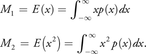
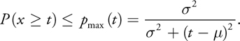
From these we can compute the mean and variance 2 of the distribution:
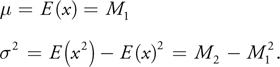
Using the variance, we can apply Chebyshev's inequality to compute an upper bound on the probability that the currently shaded surface (at depth t) is occluded:
This "one-tailed" version of Chebyshev's inequality is valid for t > . If t
 m, p max = 1 and the surface is fully lit.
The inequality gives an upper bound on the percentage-closer filtering result over an arbitrary filter region. An upper bound is advantageous to avoid self-shadowing in regions that should be fully lit. More important, Donnelly and Lauritzen 2006 show that this inequality becomes exact for a single planar occluder and single planar receiver, which is a reasonable approximation for many real scenes. In particular for a single occluder and single receiver, there is a small neighborhood in which they will be locally planar, and thus p max computed over this region will be a good approximation of the true probability.
Therefore, we can use p max directly in rendering. Listing 8-1 gives some sample code in HLSL.
Note that it is useful to clamp the minimum variance to a very small value, as we have done here, to avoid any numeric issues that may occur during filtering. Additionally, simply clamping the variance often eliminates shadow biasing issues (discussed in detail in Section 8.4.2).
8.4.1 Filtering the Variance Shadow Map
Now that the shadow map is linearly filterable, a host of techniques and algorithms are available to us. Most notably, we can simply enable mipmapping, trilinear and anisotropic filtering, and even multisample antialiasing (while rendering the shadow map). This alone significantly improves the quality compared to using standard shadow maps and constant-filter percentage-closer filtering, as shown in Figure 8-4.
)
Figure 8-4 Hardware Filtering with Variance Shadow Maps
Example 8-1. Computing p max During Scene Shading
float ChebyshevUpperBound(float2 Moments, float t)
{
  // One-tailed inequality valid if t > Moments.x
  float p = (t < = Moments.x);
  // Compute variance.
  float Variance = Moments.y – (Moments.x * Moments.x);
  Variance = max(Variance, g_MinVariance);
  // Compute probabilistic upper bound.
  float d = t – Moments.x;
  float p_max = Variance / (Variance + d * d);
  return max(p, p_max);
}
float ShadowContribution(float2 LightTexCoord, float DistanceToLight)
{
  // Read the moments from the variance shadow map.
  float2 Moments = texShadow.Sample(ShadowSampler, LightTexCoord).xy;
  // Compute the Chebyshev upper bound.
  return ChebyshevUpperBound(Moments, DistanceToLight);
}
We can do much more, however. In particular, Donnelly and Lauritzen 2006 suggests blurring the variance shadow map before shading (a simple box filter is sufficient). This approach is equivalent to neighborhood-sampled percentage-closer filtering, but it is significantly cheaper because of the use of a separable blur convolution. As discussed earlier, effectively clamping the minimum filter width like this will soften the shadow edges, helping hide magnification artifacts.
An alternative to using hardware filtering is to use summed-area tables, which also require linearly filterable data. We discuss this option in more detail in Section 8.5.
8.4.2 Biasing
In addition to providing cheap, high-quality filtering, a variance shadow map offers an elegant solution to the problem of shadow biasing.
As we discussed for percentage-closer filtering, polygons that span large depth ranges are typically a problem for shadow-mapping algorithms. Variance shadow maps, however, give us a way to represent the depth extents of a pixel by using the second moment.
Instead of considering the entire extent of a shadow map texel to be at depth , we consider it to represent a locally planar distribution, given parametrically by
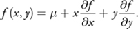
We can then compute M 2, using the linearity of the expectation operator and the fact that E(x) = E(y) = E(xy) = 0:
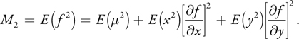
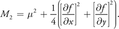
Now, representing the pixel as a symmetric Gaussian distribution with a half-pixel standard deviation yields
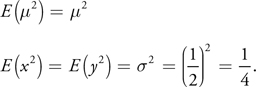
Therefore
Note that this formula reduces to simply the squared depth when the partial derivatives are both 0 (that is, when the surface is parallel to the light projection plane). Also note that no additional issues arise from increasing the filter width because the variance will automatically be computed over the entire region.
We can easily compute the moments during shadow-map rendering, using the HLSL partial derivative instructions shown in Listing 8-2.
One potential issue that remains is numeric inaccuracy. We can deal with this problem simply and entirely by clamping the minimum variance to a very small value before computing p max, as in Listing 8-1. This value is independent of the scene geometry, so it can be set once without requiring incessant tweaking. Thus, biasing alone is a compelling reason to use variance shadow maps, as demonstrated in Figure 8-5.
)
Figure 8-5 Variance Shadow Maps Resolve Biasing Issues
Example 8-2. Computing the Moments During Variance Shadow Map Rendering
float2 ComputeMoments(float Depth)
{
  float2 Moments;
  // First moment is the depth itself.
  Moments.x = Depth;
  // Compute partial derivatives of depth.
  float dx = ddx(Depth);
  float dy = ddy(Depth);
  // Compute second moment over the pixel extents.
  Moments.y = Depth * Depth + 0.25 * (dx * dx + dy * dy);
  return Moments;
}
Finally, it is usually beneficial to clamp the partial derivative portion of M 2 to avoid an excessively high variance if an occluder is almost parallel to the light direction. Hardware-generated partial derivatives become somewhat unstable in these cases and a correspondingly unstable variance can produce random, flashing pixels of light in regions that should be fully shadowed.
Many scenes can avoid this instability entirely by not using the partial derivative bias at all. If the shadow resolution is high enough, clamping the minimum variance may be all that is required to eliminate surface acne.
8.4.3 Light Bleeding
One known issue of variance shadow maps is the potential for light bleeding (light that occurs in areas that should be fully in shadow). This artifact is usually seen when the soft edge of a shadow is visible both on the first receiver (as it should be) and, to a lesser extent, on a second receiver (which should be fully occluded by the first), as shown in Figure 8-6. In Figure 8-7, the most objectionable light bleeding occurs when the ratio of a to b is large.
)
Figure 8-6 Light Bleeding
)
Figure 8-7 How Light Bleeding Occurs
The bad news is that this problem cannot be completely solved without taking more samples (which degenerates into brute-force percentage-closer filtering). This is true for any algorithm because the occluder distribution, and thus the visibility over a filter region, is a step function.
Of course, we can frequently accelerate the common filtering cases (as variance shadow mapping does nicely), but it is always possible to construct a pathological case with N distinct occluders over a filter region of N items. Any algorithm that does not sample all N values cannot correctly reconstruct the visibility function, because the ideal function is a piecewise step function with N unique pieces. As a result, an efficient shadowmap sampling algorithm that computes an exact solution over arbitrary filter regions must be adaptive.
This requirement is certainly not convenient, but it's not crippling: variance shadow mapping is actually a good building block for both an exact and an approximate shadowing algorithm. We are primarily interested in maintaining high performance and are willing to accept some infrequent physical inaccuracy, so approximate algorithms are arguably the most promising approach.
To that end, a simple modification to p max can greatly reduce the light bleeding, at the cost of somewhat darkening the penumbra regions.
An Approximate Algorithm (Light-Bleeding Reduction)
An important observation is that if a surface at depth t is fully occluded over some filter region with average depth , then t > . Therefore (t- )2 > 0, and from Chebyshev's inequality, p max < 1. Put simply, incorrect penumbrae on fully occluded surfaces will never reach full intensity.
We can remove these regions by modifying p max so that any values below some minimum intensity are mapped to 0, and the remaining values are rescaled so that they map from 0 (at the minimum intensity) to 1.
This function can be implemented trivially in HLSL, as shown in Listing 8-3.
Example 8-3. Applying a Light-Bleeding Reduction Function
float linstep(float min, float max, float v)
{
  return clamp((v – min) / (max – min), 0, 1);
}
float ReduceLightBleeding(float p_max, float Amount)
{
  // Remove the [0, Amount] tail and linearly rescale (Amount, 1].
  return linstep(Amount, 1, p_max);
}
Note that linstep() can be replaced with an arbitrary monotonically increasing continuous function over [0, 1]. For example, smoothstep() produces a nice cubic falloff function that may be desirable.
The Amount parameter is artist-editable and effectively sets the aggressiveness of the light-bleeding reduction. It is scene-scale independent, but scenes with more light bleeding will usually require a higher value. The optimal setting is related to the depth ratios of occluders and receivers in the scene. Some care should be taken with this parameter, because setting it too high will decrease shadow detail. It should therefore be set just high enough to eliminate the most objectionable light bleeding, while maintaining as much detail as possible.
In practice this solution is effectively free and works well for many scenes, as is evident in Figure 8-8. Light-bleeding reduction is therefore much more attractive than an exact adaptive algorithm for games and other performance-sensitive applications.
)
Figure 8-8 Results After Applying the Light-Bleeding Reduction Function
8.4.4 Numeric Stability
Another potential issue is numeric stability. In particular, the calculation of variance is known to be numerically unstable because of the differencing of two large, approximately equal values. Thankfully, an easy solution to the problem is to use 32-bit floating-point textures and filtering, which are supported on the GeForce 8 Series cards.
We also highly recommend using a linear depth metric rather than the post-projection z value. The latter suffers from significant precision loss as the distance from the light increases. This loss may not be a huge issue for comparison-based shadow mapping such as percentage-closer filtering, but the precision loss quickly makes the variance computation unstable. A linear metric with more uniform precision, such as the distance to the light, is more appropriate and stable.
A sample implementation of the "distance to light" depth metric for a spotlight or point light is given in Listing 8-4.
Note that the depth metric can easily be normalized to [0, 1] if a fixed-point shadowmap format is used.
For a directional light, "distance to light plane" is a suitable metric and can be obtained from the z value of the fragment position in light space. Furthermore, this z value can be computed in the vertex shader and safely interpolated, whereas the nonlinear length() function in Listing 8-4 must be computed per pixel.
We have seen no numeric stability issues when we used a linear depth metric with 32-bit floating-point numbers.
Example 8-4. Using a Linear Depth Metric for a Spotlight
// Render variance shadow map from the light's point of view.
DepthPSIn Depth_VS(DepthVSIn In)
{
  DepthPSIn Out;
  Out.Position = mul(float4(In.Position, 1), g_WorldViewProjMatrix);
  Out.PosView = mul(float4(In.Position, 1), g_WorldViewMatrix);
  return Out;
}
float4 Depth_PS(DepthPSIn In) : SV_Target
{
  float DistToLight = length(In.PosView);
  return ComputeMoments(DistToLight);
} // Render and shade the scene from the camera's point of view.
float4 Shading_PS(ShadingPSIn In) : SV_Target
{
  // Compute the distance from the light to the current fragment.
  float SurfaceDistToLight = length(g_LightPosition – In.PosWorld);
  ...
}
8.4.5 Implementation Notes
At this point, variance shadow maps are already quite usable, providing efficient filtering, cheap edge softening, and a solution to the biasing problems of standard shadow maps. Indeed, the implementation so far is suitable for use in games and other realtime applications.
To summarize, we can implement hardware variance shadow maps as follows:
- Render to the variance shadow map by using a linear depth metric (Listing 8-4), outputting depth and depth squared (Listing 8-2). Use multisample antialiasing (MSAA) on the shadow map (if it's supported).
- Optionally blur the variance shadow map by using a separable box filter.
- Generate mipmaps for the variance shadow map.
- Render the scene, projecting the current fragment into light space as usual, but using a single, filtered (anisotropic and trilinear) texture lookup into the variance shadow map to retrieve the two moments.
- Use Chebyshev's inequality to compute p max (Listing 8-1).
- Optionally, apply light-bleeding reduction to p max (Listing 8-3).
- Use p max to attenuate the light contribution caused by shadowing.
Using variance shadow maps is therefore similar to using normal shadow maps, except that blurring, multisampling, and hardware filtering can be utilized. Note, however, that some techniques used with standard shadow maps (such as the following) are inapplicable to variance shadow maps:
- Rendering "second depth" or "midpoints" into the variance shadow map will not work properly because the recovered depth distribution should represent the depths of the nearest shadow casters in light space. This is not a problem, however, because the second-depth rendering technique is used to avoid biasing issues, which can be addressed more directly with variance shadow maps (see Section 8.4.2).
- Rendering only casters (and not receivers) into the variance shadow map is incorrect! For the interpolation to work properly, the receiving surface must be represented in the depth distribution. If it is not, shadow penumbrae will be improperly sized and fail to fade smoothly from light to dark.
Projection-warping and frustum-partitioning techniques, however, are completely compatible with VSMs. Indeed, the two techniques complement one another. Variance shadow maps hide many of the artifacts introduced by warping or splitting the frustum, such as discontinuities between split points and swimming along shadow edges when the camera moves.
8.4.6 Variance Shadow Maps and Soft Shadows
Moving forward, we address a few issues with using hardware filtering. First, highprecision hardware filtering may not be available. More important, however, we want per-pixel control over the filter region.
As we have seen earlier, clamping the minimum filter width softens shadow edges. Several recent soft shadows algorithms have taken advantage of this capability by choosing the filter width dynamically, based on an estimation of the "blocker depth." This approach can produce convincing shadow penumbrae that increase in size as the distance between the blocker and receiver increases.
Unfortunately, we cannot use blurring to clamp the minimum filter width in this case, because that width changes per pixel, based on the result of the blocker search. We can certainly clamp the mipmap level that the hardware uses, but using mipmapping to blur in this manner produces extremely objectionable boxy artifacts, as shown in Figure 8-9. There is some potential for obtaining better results by using a high-order filter to manually generate the mipmap levels, which is a promising direction for future work.
)
Figure 8-9 Boxy Artifacts Caused by Mipmap Level-of-Detail Clamping
In the best of circumstances, we would have a filtering scheme that allows us to choose the filter size dynamically per pixel, ideally at constant cost and without dynamic branching. This capability is exactly what summed-area tables give us.
8.5 Summed-Area Variance Shadow Maps
Summed-area tables were introduced by Crow 1984 to accelerate texture filtering. Using a source texture with elements a[i, j], we can build a summed-area table t[i, j ] so that
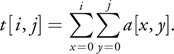
In other words, each element in the SAT is the sum of all texture elements in the rectangle above and to the left of the element (or below, if you like your origin in the bottom left). Figure 8-10 shows an example of some arbitrary data and the associated summed-area table.
)
Figure 8-10 Sample Data and the Associated Summed-Area Table
The sum of any rectangular region can then be determined in constant time:

We can easily compute the average over this region by dividing by the number of pixels in the region. Bilinear interpolation can be used when sampling the corners, producing a smooth gradient.
Note that this formula is inclusive on the "max" sides of the rectangle, but exclusive on the "min" sides. Subtracting 1 from the coordinates before lookup will produce the more common min-inclusive/max-exclusive policy.
In the example from Figure 8-10, we can compute the sum or average over the highlighted data rectangle by querying the highlighted values from the SAT (in this example, we're being inclusive on both sides for simplicity). This yields
|
s = 28 - 8 - 6 + 2 = 16, |
which is the correct sum over the highlighted data region. Dividing by the number of elements in the region (4) gives the correct average of 4.
Summed-area tables give us the ability to sample arbitrary rectangular regions, which is sufficient for our purposes. They can, however, be extended to adaptively sample nonrectangular regions (Glassner 1986).
8.5.1 Generating Summed-Area Tables
We want to generate the summed-area table on the GPU to achieve better performance and to avoid excessive data movements. Two algorithms in particular are potentially suitable: line-by-line and recursive doubling.
The line-by-line approach is basically a running sum, performed one dimension at a time. On the GPU this algorithm can be implemented by working one line at a time, adding the current line to the previous sum. The disadvantage of this method is that it requires (width+ height) passes.
An alternative approach to summed-area table generation on the GPU is recursive doubling, as proposed by Hensley et al. 2005. Refer to that publication for a complete description of the algorithm. An implementation is also available as part of the sample code accompanying this book.
8.5.2 Numeric Stability Revisited
Summed-area tables burn precision fairly quickly: log(width x height) bits. A 512x512 SAT, therefore, consumes 18 bits of precision (in the worst case), leaving only 5 bits of the 23-bit mantissa for the data itself! The average case is not this catastrophic, but using summed-area tables significantly decreases the effective precision of the underlying data.
Luckily, there are a few tricks we can use to increase the precision to an acceptable level. Hensley et al. 2005 gave a number of suggestions to improve precision for floatingpoint summed-area tables. One recommendation is to bias each of the elements by –0.5 before generating the SAT, and to unbias after averaging over a region. This approach effectively gains an extra bit of precision from the sign bit. For images (in our case, shadow maps) that contain a highly nonuniform distribution of data, biasing by the mean value of the data can produce even greater gains. Additionally, the authors suggest using an "origin-centered" SAT to save two more bits, at the cost of increased complexity. This is a particularly useful optimization for spotlights because it pushes the areas of low precision out to the four corners of the shadow projection so that any artifacts will be largely hidden by the circular spotlight attenuation cone.
A trick suggested by Donnelly and Lauritzen 2006 is also useful here: distributing precision into multiple components. Instead of storing a two-component variance shadow map, we store four components, distributing each of the first two moments into two components. This precision splitting cannot be done arbitrarily; to work properly with linear filtering, it must be a linear operation. Nevertheless, Listing 8-5 gives a sample implementation that works fairly well in practice.
Example 8-5. Distributing Floating-Point Precision
// Where to split the value. 8 bits works well for most situations.
float g_DistributeFactor = 256;
float4 DistributePrecision(float2 Moments)
{
  float FactorInv = 1 / g_DistributeFactor;
  // Split precision
  float2 IntPart;
  float2 FracPart = modf(Value * g_DistributeFactor, IntPart);
  // Compose outputs to make reconstruction cheap.
  return float4(IntPart * FactorInv, FracPart);
}
float2 RecombinePrecision(float4 Value)
{
  float FactorInv = 1 / g_DistributeFactor;
  return (Value.zw * FactorInv + Value.xy);
}
This step, of course, doubles the storage and bandwidth requirements of summed-area variance shadow maps, but the resulting implementation can still outperform bruteforce percentage-closer filtering in many situations, as we show in Section 8.5.3.
Another option, made available by the GeForce 8 Series hardware, is to use 32-bit integers to store the shadow map. Storing the shadow map this way saves several bits of precision that would otherwise be wasted on the exponent portion of the float (which we do not use).
When we use integers, overflow is a potential problem. To entirely avoid overflow, we must reserve log(width x height) bits for accumulation. Fortunately, the overflow behavior in Direct3D 10 (wraparound) actually works to our advantage. In particular, if we know the maximum filter size that we will ever use is M x x M y , we need only reserve log(M x x M y ) bits. Because a fairly conservative upper bound can often be put on filter sizes, plenty of bits are left for the data. In practice, this solution works extremely well even for large shadow maps and does not require any tricks such as distributing precision.
A final alternative, once hardware support is available, is to use double-precision floating-point numbers to store the moments. The vast precision improvement of double precision (52 bits versus 23 bits) will eliminate any issues that numeric stability causes.
8.5.3 Results
Figure 8-11 shows an image rendered using a 512x512 summed-area variance shadow map. Note the lack of any visible aliasing. Figure 8-12 shows hard and soft shadows obtained simply by varying the minimum filter width. The performance of the technique is independent of the filter width, so arbitrarily soft shadows can be achieved without affecting the frame rate.
)
Figure 8-11 Shadows Using Summed-Area Variance Shadow Maps
)
Figure 8-12 Hard-Edged and Soft-Edged Shadows Using Summed-Area Variance Shadow Maps
The technique is also very fast on modern hardware. Figure 8-13 compares the performance of PCF (with hardware acceleration), blurred VSMs (with and without shadow multisampling), and SAVSMs. We chose a simple test scene to evaluate relative performance, because all of these techniques operate in image space and are therefore largely independent of geometric complexity.
)
Figure 8-13 Relative Frame Times of PCF, VSM, and SAVSM
Clearly, standard blurred variance shadow maps are the best solution for constant filter widths. Even when multisampling is used, VSMs are faster than the competition. Note that the cost of blurring the variance shadow map is theoretically linear in the filter width, but because modern hardware can perform these separable blurs extremely quickly, the reduced performance is not visible unless extremely large filters are used.
For dynamic filter widths, summed-area variance shadow maps have a higher setup cost than percentage-closer filtering (generating the SAT). However, this cost is quickly negated by the higher sampling cost of PCF, particularly for larger minimum filter sizes (such as softer shadows). In our experience, a minimum filter width of at least four is required to eliminate the most objectionable aliasing artifacts of shadow maps, so SAVSM is the obvious winner. We expect that additional performance improvements can be realized with more aggressive optimization.
8.6 Percentage-Closer Soft Shadows
Now that we have an algorithm that can filter arbitrary regions at constant cost, we are ready to use SAVSMs to produce plausible soft shadows. Any algorithm that does a PCF-style sampling over the shadow map is a potential candidate for integration.
One such algorithm, proposed by Fernando 2005, is percentage-closer soft shadows (PCSS), which is particularly attractive because of its simplicity. PCSS works in three steps: (1) the blocker search, (2) penumbra size estimation, and (3) shadow filtering.
8.6.1 The Blocker Search
The blocker search samples a search region around the current shadow texel and finds the average depth of any blockers in that region. The search region size is proportional to both the light size and the distance to the light. A sample is considered a blocker if it is closer to the light than the current fragment (using the standard depth test).
One unfortunate consequence of this step is that it will reintroduce the biasing issues of PCF into our soft shadows algorithm, because of the depth test. Moreover, taking many samples over some region of the shadow map is disappointing after having worked so hard to get constant-time filtering.
8.6.2 Penumbra Size Estimation
This step of the algorithm uses the previously computed blocker depth to estimate the size of the penumbra, based on a parallel planes approximation. We list the formula here and refer the reader to Fernando 2005 for the derivation based on similar triangles:
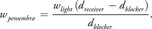
Here, w light refers to the light size.
8.6.3 Shadow Filtering
During filtering, summed-area variance shadow maps can be used directly, improving the quality and performance of the algorithm over the uniform grid percentage-closer filtering that was used in the original implementation.
8.6.4 Results
Figure 8-14 shows a side-by-side comparison of PCSS using percentage-closer filtering (left) and summed-area variance shadow maps (right) for the filtering step. The sample scene is especially difficult, forcing both implementations to take many samples (64) during the blocker search step. Regardless of this equalizing bottleneck, the SAVSM implementation outperformed the PCF implementation by a reasonable margin: 40 frames/sec versus 25 frames/sec at 1600x1200. Furthermore, the image quality of the PCF implementation was inferior because it sparsely sampled the filter region.
)
Figure 8-14 Plausible Soft Shadows Using PCSS
Although preliminary, these results imply that summed-area variance shadow maps are well suited to usage in a soft shadows algorithm. We are looking forward to further research in this area.
8.7 Conclusion
We have discussed the topic of shadow-map filtering in detail and have provided solutions to many associated problems, such as minification aliasing, biasing, and soft shadows.
We have shown that variance shadow maps are quite useful and are a promising direction for future research. That said, standard blurred variance shadow maps, combined with a light-bleeding reduction function, are extremely fast and robust, and they provide excellent quality. We highly recommend using this implementation for shadow filtering in most applications, which do not require per-pixel filter width control.
For plausible soft shadows, variance shadow maps have also proven useful. Combined with summed-area tables, they provide constant-time filtering of arbitrary rectangular regions.
In conclusion, we hope this chapter has offered useful solutions and that it will motivate future research into variance shadow maps and real-time shadow-filtering algorithms in general.
8.8 References
Crow, Franklin. 1977. "Shadow Algorithms for Computer Graphics." In Computer Graphics (Proceedings of SIGGRAPH 1977) 11(2), pp. 242–248.
Crow, Franklin. 1984. "Summed-Area Tables for Texture Mapping." In Computer Graphics (Proceedings of SIGGRAPH 1984) 18(3), pp. 207–212.
Donnelly, William, and Andrew Lauritzen. 2006. "Variance Shadow Maps." In Proceedings of the Symposium on Interactive 3D Graphics and Games 2006, pp. 161–165.
Fernando, Randima. 2005. "Percentage-Closer Soft Shadows." In SIGGRAPH 2005 Sketches.
Glassner, Andrew. 1986. "Adaptive Precision in Texture Mapping." In Computer Graphics (Proceedings of SIGGRAPH 1986) 20(4), pp. 297–306.
Hensley, Justin, Thorsten Scheuermann, Greg Coombe, Montek Singh, and Anselmo Lastra. 2005. "Fast Summed-Area Table Generation and Its Applications." Computer Graphics Forum 24(3), pp. 547–555.
Kilgard, Mark. 2001. "Shadow Mapping with Today's OpenGL Hardware." Presentation at CEDEC 2001.
Martin, Tobias, and Tiow-Seng Tan. 2004. "Anti-aliasing and Continuity with Trapezoidal Shadow Maps." In Eurographics Symposium on Rendering Proceedings 2004, pp. 153–160.
Reeves, William, David Salesin and Robert Cook. 1987. "Rendering Antialiased Shadows with Depth Maps." In Computer Graphics (Proceedings of SIGGRAPH 1987) 21(3), pp. 283–291.
Stamminger, Marc, and George Drettakis. 2002. "Perspective Shadow Maps." In ACM Transactions on Graphics (Proceedings of SIGGRAPH 2002) 21(3), pp. 557–562.
Williams, Lance. 1978. "Casting Curved Shadows on Curved Surfaces." In Computer Graphics (Proceedings of SIGGRAPH 1978) 12(3), pp. 270–274.
Wimmer, Michael, D. Scherzer, and Werner Purgathofer. 2004. "Light Space Perspective Shadow Maps." In Proceedings of the Eurographics Symposium on Rendering 2004, pp. 143–152.
Many people deserve thanks for providing helpful ideas, suggestions, and feedback, including William Donnelly (University of Waterloo), Michael McCool (RapidMind), Mandheerej Nandra (Caltech), Randy Fernando (NVIDIA), Kevin Myers (NVIDIA), and Hubert Nguyen (NVIDIA). Additional thanks go to Chris Iacobucci (Silicon Knights) for the car and commando 3D models and textures.
- Contributors
- Foreword
- Part I: Geometry
-
- Chapter 1. Generating Complex Procedural Terrains Using the GPU
- Chapter 2. Animated Crowd Rendering
- Chapter 3. DirectX 10 Blend Shapes: Breaking the Limits
- Chapter 4. Next-Generation SpeedTree Rendering
- Chapter 5. Generic Adaptive Mesh Refinement
- Chapter 6. GPU-Generated Procedural Wind Animations for Trees
- Chapter 7. Point-Based Visualization of Metaballs on a GPU
- Part II: Light and Shadows
-
- Chapter 8. Summed-Area Variance Shadow Maps
- Chapter 9. Interactive Cinematic Relighting with Global Illumination
- Chapter 10. Parallel-Split Shadow Maps on Programmable GPUs
- Chapter 11. Efficient and Robust Shadow Volumes Using Hierarchical Occlusion Culling and Geometry Shaders
- Chapter 12. High-Quality Ambient Occlusion
- Chapter 13. Volumetric Light Scattering as a Post-Process
- Part III: Rendering
-
- Chapter 14. Advanced Techniques for Realistic Real-Time Skin Rendering
- Chapter 15. Playable Universal Capture
- Chapter 16. Vegetation Procedural Animation and Shading in Crysis
- Chapter 17. Robust Multiple Specular Reflections and Refractions
- Chapter 18. Relaxed Cone Stepping for Relief Mapping
- Chapter 19. Deferred Shading in Tabula Rasa
- Chapter 20. GPU-Based Importance Sampling
- Part IV: Image Effects
-
- Chapter 21. True Impostors
- Chapter 22. Baking Normal Maps on the GPU
- Chapter 23. High-Speed, Off-Screen Particles
- Chapter 24. The Importance of Being Linear
- Chapter 25. Rendering Vector Art on the GPU
- Chapter 26. Object Detection by Color: Using the GPU for Real-Time Video Image Processing
- Chapter 27. Motion Blur as a Post-Processing Effect
- Chapter 28. Practical Post-Process Depth of Field
- Part V: Physics Simulation
-
- Chapter 29. Real-Time Rigid Body Simulation on GPUs
- Chapter 30. Real-Time Simulation and Rendering of 3D Fluids
- Chapter 31. Fast N-Body Simulation with CUDA
- Chapter 32. Broad-Phase Collision Detection with CUDA
- Chapter 33. LCP Algorithms for Collision Detection Using CUDA
- Chapter 34. Signed Distance Fields Using Single-Pass GPU Scan Conversion of Tetrahedra
- Chapter 35. Fast Virus Signature Matching on the GPU
- Part VI: GPU Computing
-
- Chapter 36. AES Encryption and Decryption on the GPU
- Chapter 37. Efficient Random Number Generation and Application Using CUDA
- Chapter 38. Imaging Earth's Subsurface Using CUDA
- Chapter 39. Parallel Prefix Sum (Scan) with CUDA
- Chapter 40. Incremental Computation of the Gaussian
- Chapter 41. Using the Geometry Shader for Compact and Variable-Length GPU Feedback
- Preface