GPU Gems 3

GPU Gems 3 is now available for free online!

The CD content, including demos and content, is available on the web and for download.

You can also subscribe to our Developer News Feed to get notifications of new material on the site.

Chapter 7. Point-Based Visualization of Metaballs on a GPU

Kees van Kooten
Playlogic Game Factory

Gino van den Bergen
Playlogic Game Factory

Alex Telea
Eindhoven University of Technology

In this chapter we present a technique for rendering metaballs on state-of-the-art graphics processors at interactive rates. Instead of employing the marching cubes algorithm to generate a list of polygons, our method samples the metaballs' implicit surface by constraining free-moving particles to this surface. Our goal is to visualize the metaballs as a smooth surface by rendering thousands of particles, with each particle covering a tiny surface area. To successfully apply this point-based technique on a GPU, we solve three basic problems. First, we need to evaluate the metaballs' implicit function and its gradient per rendered particle in order to constrain the particles to the surface. For this purpose, we devised a novel data structure for quickly evaluating the implicit functions in a fragment shader. Second, we need to spread the particles evenly across the surface. We present a fast method for performing a nearest-neighbors search on each particle that takes two rendering passes on a GPU. This method is used for computing the repulsion forces according to the method of smoothed particle hydrodynamics. Third, to further accelerate particle dispersion, we present a method for transferring particles from high-density areas to low-density areas on the surface.

7.1 Metaballs, Smoothed Particle Hydrodynamics, and Surface Particles

The visualization of deformable implicit surfaces is an interesting topic, as it is aimed at representing a whole range of nonrigid objects, ranging from soft bodies to water and gaseous phenomena. Metaballs, a widely used type of implicit surface invented by Blinn in the early 1980s (Blinn 1982), are often used for achieving fluid-like appearances.

The concept of metaballs is closely related to the concept of smoothed particle hydrodynamics (SPH) (Müller et al. 2003), a method used for simulating fluids as clouds of particles. Both concepts employ smooth scalar functions that map points in space to a mass density. These scalar functions, referred to as smoothing kernels, basically represent point masses that are smoothed out over a small volume of space, similar to Gaussian blur in 2D image processing. Furthermore, SPH-simulated fluids are visualized quite naturally as metaballs. This chapter does not focus on the dynamics of the metaballs themselves. We are interested only in the visualization of clouds of metaballs in order to create a fluid surface. Nevertheless, the proposed techniques for visualizing metaballs rely heavily on the SPH method. We assume that the metaballs, also referred to as fluid atoms, are animated on the CPU either by free-form animation techniques or by physics-based simulation. Furthermore, we assume that the dynamics of the fluid atoms are interactively determined, so preprocessing of the animation sequence of the fluid such as in Vrolijk et al. 2004 is not possible in our case.

The fluid atoms in SPH are basically a set of particles, defining the implicit metaball surface by its spatial configuration. To visualize this surface, we use a separate set of particles called surface particles, which move around in such a way that they remain on the implicit surface defined by the fluid atoms. These particles can then be rendered as billboards or oriented quads, as an approximation of the fluid surface.

7.1.1 A Comparison of Methods

The use of surface particles is not the most conventional way to visualize implicit surfaces. More common methodologies are to apply the marching cubes algorithm (Lorenson and Cline 1987) or employ ray tracing (Parker et al. 1998). Marching cubes discretizes the 3D volume into a grid of cells and calculates for every cell a set of primitives based on the implicit-function values of its corners. These primitives interpolate the intersection of the implicit surface with the grid cells. Ray tracing shoots rays from the viewer at the surface to determine the depth and color of the surface at every pixel. Figure 7-1 shows a comparison of the three methods.

Figure 7-1 Methods of Visualizing Implicit Surfaces

Point-based methods (Witkin and Heckbert 1994) have been applied much less frequently for visualizing implicit surfaces. The most likely reason for this is the high computational cost of processing large numbers of particles for visualization. Other techniques such as ray tracing are computationally expensive as well but are often easier to implement on traditional CPU-based hardware and therefore a more obvious choice for offline rendering.

With the massive growth of GPU processing power, implicit-surface visualization seems like a good candidate to be offloaded to graphics hardware. Moreover, the parallel nature of today's GPUs allows for a much faster advancement in processing power over time, giving GPU-run methods an edge over CPU-run methods in the future. However, not every implicit-surface visualization technique is easily modified to work in a parallel environment. For instance, the marching cubes algorithm has a complexity in the order of the entire volume of a metaball object; all grid cells have to be visited to establish a surface (Pascucci 2004). An iterative optimization that walks over the surface by visiting neighboring grid cells is not suitable for parallelization. Its complexity is therefore worse than the point-based method, which has to update all surface particle positions; the number of particles is linearly related to the fluid surface area.

By their very nature, particle systems are ideal for exploiting temporal coherence. Once the positions of surface particles on a fluid surface are established at a particular moment in time, they have to be moved only a small amount to represent the fluid surface a fraction of time later. Marching cubes and ray tracing cannot make use of this characteristic. These techniques identify the fluid surface from scratch every time again.

7.1.2 Point-Based Surface Visualization on a GPU

We propose a method for the visualization of metaballs, using surface particles. Our primary goal is to cover as much of the fluid surface as possible with the surface particles, in the least amount of time. We do not focus on the actual rendering of the particles itself; we will only briefly treat blending of particles and shader effects that create a more convincing surface.

Our method runs almost entirely on a GPU. By doing so, we avoid a lot of work on the CPU, leaving it free to do other tasks. We still need the CPU for storing the positions and velocities of the fluid atoms in a form that can be processed efficiently by a fragment shader. All other visualization tasks are offloaded to the GPU. Figure 7-2 gives an overview of the process.

Figure 7-2 The Fluid Simulation Loop Performed on the CPU Together with the Fluid Visualization Loop Performed on the GPU

Our approach is based on an existing method by Witkin and Heckbert (1994). Here, an implicit surface is sampled by constraining particles to the surface and spreading them evenly across the surface. To successfully implement this concept on GPUs with at least Shader Model 3.0 functionality, we need to solve three problems:

First, we need to efficiently evaluate the implicit function and its gradient in order to constrain the particles on the fluid surface. To solve this problem, we choose a data structure for quickly evaluating the implicit function in the fragment shader. This data structure also optionally minimizes the GPU workload in GPU-bound scenarios. We describe this solution in Section 7.2.

Second, we need to compute the repulsion forces between the particles in order to obtain a uniform distribution of surface particles. A uniform distribution of particles is of vital importance because on the one hand, the amount of overlap between particles should be minimized in order to improve the speed of rendering. On the other hand, to achieve a high visual quality, the particles should cover the complete surface and should not allow for holes or cracks. We solve this problem by computing repulsion forces acting on the surface particles according to the SPH method. The difficulty in performing SPH is querying the particle set for nearest neighbors. We provide a novel algorithm for determining the nearest neighbors of a particle in the fragment shader. We present the computation of repulsion forces in Section 7.3.

Finally, we add a second distribution algorithm, because the distribution due to the repulsion forces is rather slow, and it fails to distribute particles to disconnected regions. This global dispersion algorithm accelerates the distribution process and is explained in Section 7.4.

In essence, the behavior of the particles can be defined as a fluid simulation of particles moving across an implicit surface. GPUs have been successfully applied for similar physics-based simulations of large numbers of particles (Latta 2004). However, to our knowledge, GPU-based particle systems in which particles influence each other have not yet been published.

7.2 Constraining Particles

To constrain particles to an implicit surface generated by fluid atoms, we will restrict the velocity of all particles such that they will only move along with the change of the surface. For the moment, they will be free to move tangentially to the surface, as long as they do not move away from it. Before defining the velocity equation for surface particles, we will start with the definition of the function yielding our implicit surface.

7.2.1 Defining the Implicit Surface

For all of the following sections, we define a set of fluid atoms {j: 1 j m}—the metaballs—simulated on the CPU with positions a _j , and a set of surface particles {i: 1 i n} with positions p _i . The fluid atoms define a fluid surface, which we are going to visualize using the fluid particles. The surface is computed as an isosurface of a fluid density function F(x, ). The function depends on the evaluation position x and a state vector representing the concatenation of all fluid atom positions. Following the SPH model of Müller et al. 2003, the fluid density is given by

Equation 1

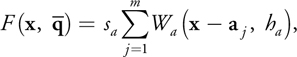
using smoothing kernels W _a (r, h _a ) to distribute density around every atom position by a scaling factor s _a . The smoothing kernel takes a vector r to its center, and a radius h _a in which it has a nonzero contribution to the density field. Equation 1 is the sum of these smoothing kernels with their centers placed at different positions. The actual smoothing kernel function can take different forms; the following is the one we chose, which is taken from Müller et al. 2003 and illustrated in Figure 7-3.

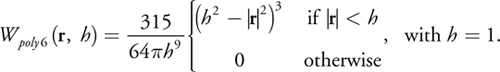
Figure 7-3 The Smoothing Kernel

7.2.2 The Velocity Constraint Equation

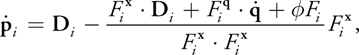
To visualize the fluid isosurface described in Section 7.2.1, we will use the point-based method of Witkin and Heckbert 1994. This method proposes both an equation for moving particles along with the surface and an equation for moving the surface along with the particles. We require only the former, shown here as Equation 2. This equation yields the constrained velocity of a surface particle; the velocity will always be tangent to the fluid surface as the surface changes.

Equation 2

where is the constrained velocity of particle i obtained by application of the equation; D _i is a desired velocity that we may choose; is the concatenation of all fluid atom velocities; F _i is the density field F(x, ) evaluated at particle position p _i ; and are the derivatives of the density field F(x, ) with respect to x and , respectively, evaluated at particle position p _i as well.

We choose the desired velocity D _i in such a way that particles stay at a fixed position on the fluid surface as much as possible. The direction and size of changes in the fluid surface at a certain position x depend on both the velocity of the fluid atoms influencing the density field at x, as well as the gradient magnitude of their smoothing kernel at x. This results in the definition of D _i , shown in Equation 3. We denote this component of D _i by because we will add another component to D _i in Section 7.3.

Equation 3

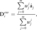
with

equals

evaluated at particle position p _i , which equals

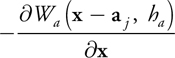
evaluated at p _i (omitting s _a ). This is simply the negative gradient of a single smoothing kernel centered at a _j , evaluated at p _i . Summarizing, is a weighted sum of atom velocities with their weight determined by the length of .

To put the preceding result in perspective: In our simulation of particle movement, the velocity of the particles will be defined by Equation 2. The equation depends on the implicit function with its gradients at particle positions and a desired velocity D _i , which in turn consists of a number of components, and These components are influenced by fluid atom velocities and surface particle repulsion forces, respectively. The first component is defined by Equation 3; the second component is discussed in Section 7.3. The implementation of the algorithm appears in Listing 7-1.

Example 7-1. Implementation Part 1: Pseudocode of a Fragment Program Simulating the Velocity of a Surface Particle

 void mainvel() {   //Perform two lookups to find the particle position and velocity    //in the corresponding textures.   position = f3tex2D(pos_texture, particle_coord);   velocity = f3tex2D(vel_texture, particle_coord);   //Compute the terms of Equations 2 and 3.   for each fluid atom  //See Listing 7-2.   {     fluid_atom_pos, fluid_atom_vel; //See Listing 7-2 for data lookup.     r = position - fluid_atom_pos;     if |r| within atomradius     {       //Compute density "F".       density += NORM_SMOOTHING_NORM * (atomradius - |r|*|r|)^3;       //The gradient "Fx"       gradient_term = 6 * NORM_SMOOTHING_NORM * r *                       (atomradius – |r|*|r|)^2;       gradient -= gradient_term;       //The dot product of atom velocity with       //the gradient "dot(Fq,q')"       atomvelgradient += dot(gradient_term, fluid_atom_vel);       //The environment velocity "wj*aj"       vel_env_weight += |gradient_term|;       vel_environment += vel_env_weight * fluid_atom_vel;     }   }   //Compute final environment velocity.   vel_environment /= vel_env_weight;   //Compute repulsion velocity (incorporates velocity).    //See Listing 7-4 for querying the repulsion force hash.    //Compute desired velocity.   vel_desired = vel_environment + vel_repulsion;   //Compute the velocity constraint from Equation 2.   terms = - dot(gradient, vel_desired) //dot(Fx,D)           - atomvelgradient            //dot(Fq,q')           - 0.5f * density;            //phi * F   newvelocity = terms / dot(gradient, gradient) * gradient;   //Output the velocity, gradient, and density. }

7.2.3 Computing the Density Field on the GPU

Now that we have established a velocity constraint on particles with Equation 2, we will discuss a way to calculate this equation efficiently on the GPU. First, note that the function can be reconstructed using only fluid atom positions and fluid atom velocities—the former applies to terms F _i , , , and ; the latter to and . Therefore, only atom positions and velocities have to be sent from the SPH simulation on the CPU to the GPU. Second, instead of evaluating every fluid atom position or velocity to compute Equation 1 and its derivatives—translating into expensive texture lookups on the GPU—we aim to exploit the fact that atoms contribute nothing to the density field outside their influence radius h _a .

For finding all neighboring atoms, we choose to use the spatial hash data structure described in Teschner et al. 2003. An advantage of a spatial hash over tree-based spatial data structures is the constant access time when querying the structure. A tree traversal requires visiting nodes possibly not adjacent in video memory, which would make the procedure unnecessarily expensive.

In the following, we present two enhancements of the hash structure of Teschner et al. 2003 in order to make it suitable for application on a GPU. We modify the hash function for use with floating-point arithmetic, and we adopt a different way of constructing and querying the hash.

7.2.4 Choosing the Hash Function

First, the spatial hash structure we use is different in the choice of the hash function. Because we have designed this technique to work on Shader Model 3.0 hardware, we cannot rely on real integer arithmetic, as in Shader Model 4.0. As a result, we are restricted to using the 23 bits of the floating-point mantissa. Therefore, we use the hash function from Equation 4.

Equation 4

with

where the three-vector of integers B(x, y, z) is the discretization of the point (x, y, z) into grid cells, with B _x , B _y , and B _z its x, y, and z components, and s the grid cell size. We have added the constant term c to eliminate symmetry around the origin. The hash function H(x, y, z) maps three-component vectors to an integer representing the index into an array of hash buckets, with hs being the hash size and p ₁, p ₂, and p ₃ large primes. We choose primes 11,113, 12,979, and 13,513 to make sure that the world size could still be reasonably large without exceeding the 23 bits available while calculating the hash function.

7.2.5 Constructing and Querying the Hash

Before highlighting the second difference of our hash method, an overview of constructing and querying the hash is in order. We use the spatial hash to carry both the fluid atom positions and the velocities, which have to be sent from the fluid simulation on the CPU to the fluid visualization on the GPU. We therefore perform its construction on the CPU, while querying happens on the GPU.

The implementation of the spatial hash consists of two components: a hash index table and atom attribute pools. The hash index table of size hs indexes the atom attribute pools storing the fluid atoms' positions and velocities. Every entry e in the hash index table corresponds to hash bucket e, and the information in the hash index table points to the bucket's first attribute element in the atom attribute pools, together with the number of elements present in that bucket. Because the spatial hash is used to send atom positions and velocities from the CPU to the GPU, we perform construction on the CPU, while querying happens on the GPU. Figure 7-4 demonstrates the procedure of querying this data structure on the GPU.

Figure 7-4 Querying the Hash Table

We will now describe the second difference compared to Teschner et al. 2003, relating to the method of hash construction. The traditional method of constructing a spatial hash adds every fluid atom to the hash table once, namely to the hash bucket to which its position maps. When the resulting structure is used to find neighbors, the traditional method would perform multiple queries per fluid atom: one for every grid cell intersecting a sphere around its position with the radius of the fluid atoms. This yields all fluid atoms influencing the density field at its position. However, we use an inverted hash method: the fluid atom is added to the hash multiple times, for every grid cell intersecting its influence area. Then, the GPU has to query a hash bucket only once to find all atoms intersecting or encapsulating the grid cell. The methods are illustrated in Figure 7-5. Listing 7-2 contains the pseudocode.

Figure 7-5 Comparing Hash Methods

Performance-wise, the inverted hash method has the benefit of requiring only a single query on the GPU, independent of the chosen grid cell size. When decreasing the hash cell size, we can accomplish a better approximation of a grid cell with respect to the fluid atoms that influence the positions inside it. These two aspects combined minimize the number of data lookups a GPU has to perform in texture memory. However, construction time on the CPU increases with smaller grid cell sizes, because the more grid cells intersect a fluid atom's influence radius, the higher the number of additions of a single atom to the hash. The traditional hash method works the other way around: a decreasing grid cell size implies more queries for the GPU, while an atom will always be added to the hash only once by the CPU. Hardware configurations bottlenecked by the GPU should therefore opt for the inverted hash method, while configurations bottlenecked by the CPU should opt for the traditional hash method.

Example 7-2. Implementation Part 2: Pseudocode for Querying the Hash

 float hash(float3 point) {   float3 discrete = (point + 100.0) * INV_CELL_SIZE;   discrete = floor(discrete) * float3(11113.0f, 12979.0f, 13513.0f);   float result = abs(discrete.x + discrete.y + discrete.z);   return fmod(result, NUM_BUCKETS); } void mainvel(   . . .   const uniform float hashindex_dim, //Width of texRECT   const uniform float hashdata_dim,   const uniform samplerRECT hsh_idx_tex : TEXUNIT4,   const uniform samplerRECT hsh_dta_tex_pos : TEXUNIT5,   const uniform samplerRECT hsh_dta_tex_vel : TEXUNIT6,   . . . ) {   //Other parts of this program discussed in Section 7.2.2    //Compute density F, its gradient Fx, and dot(Fq,q').    //Calculate hashvalue; atomrange stores length and 1D index    //into data table.   float hashvalue = hash(position);   float2 hsh_idx_coords = float2(fmod(hashvalue, hashindex_dim),                                  hashvalue / hashindex_dim);   float4 atomrange = texRECT(hsh_idx_texture, hsh_idx_coords);   float2 hashdata = float2(fmod(atomrange.y, hashdata_dim),                            atomrange.y / hashdata_dim);   //For each fluid atom   for(int i = 0; i < atomrange.x; i++)   {     //Get the fluid atom position and velocity from the hash.     float3 fluid_atom_pos = f3texRECT(hsh_dta_texture_pos, hashdata);     float3 fluid_atom_vel = f3texRECT(hsh_dta_texture_vel, hashdata);     //See Listing 7-1 for the contents of the loop.   } }

7.3 Local Particle Repulsion

On top of constraining particles to the fluid surface, we require them to cover the entire surface area. To obtain a uniform distribution of particles over the fluid surface, we adopt the concept of repulsion forces proposed in Witkin and Heckbert 1994. The paper defines repulsion forces acting on two points in space by their distance; the larger the distance, the smaller the repulsion force. Particles on the fluid surface have to react to these repulsion forces. Thus they are not free to move to every position on the surface anymore.

7.3.1 The Repulsion Force Equation

We alter the repulsion function from Witkin and Heckbert 1994 slightly, for we would like particles to have a bounded region in which they influence other particles. To this end, we employ the smoothing kernels from SPH (Müller et al. 2003) once again, which have been used similarly for the fluid density field of Equation 1. Our new function is defined by Equation 5 and yields a density field that is the basis for the generation of repulsion forces.

Equation 5

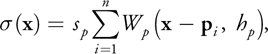
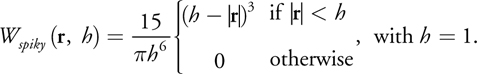
where W _p is the smoothing kernel chosen for surface particles, h _p is the radius of the smoothing kernel in which it has a nonzero contribution to the density field, and s _p is a scaling factor for surface particles. Our choice for W _p is again taken from Müller et al. 2003 and presented in the equation below, and in Figure 7-6. We can use this smoothing kernel to calculate both densities and repulsion forces, because it has a nonnegative gradient as well.

Figure 7-6 The Smoothing Kernel Used for Surface Particles

The repulsion force at a particle position p _i is the negative gradient of the density field.

Equation 6

To combine the repulsion forces with our velocity constraint equation, the repulsion force is integrated over time to form a desired repulsion velocity . We can use simple Euler integration:

Equation 7

where t = t _new - t _old .

The final velocity D _i is obtained by adding and :

Equation 8

The total desired velocity D _i is calculated and used in Equation 2 every time the surface particle velocity is constrained on the GPU.

7.3.3 Nearest Neighbors on a GPU

Now that we have defined the repulsion forces acting on surface particles with Equation 6, we are once again facing the challenge of calculating them efficiently on the GPU. Just as we did with fluid atoms influencing a density field, we will exploit the fact that a particle influences the density field in only a small neighborhood around it. A global data structure will not be a practical solution in this case; construction would have to take place on the GPU, not on the CPU. The construction of such a structure would rely on sorting or similar kinds of interdependent output, which is detrimental to the execution time of the visualization. For example, the construction of a data structure like the spatial hash in Section 7.2.3 would consist of more than one pass on the GPU, because it requires variable-length hash buckets.

Our way around the limitation of having to construct a data structure is to use a render target on the video card itself. We use it to store floating-point data elements, with construction being performed by the transformation pipeline. By rendering certain primitives at specific positions while using shader programs, information from the render target can be queried and used during the calculation of repulsion forces.

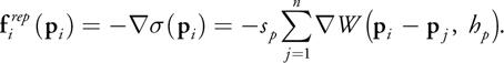
The algorithm works in two steps:

First Pass

Set up a transformation matrix M representing an orthogonal projection, with a viewport encompassing every surface particle, and a float4 render target.
Render surface particles to the single pixel to which their center maps.
Store their world-space coordinate at the pixel in the frame buffer.
Save the render target as texture "Image 1," as shown in Figure 7-7a.

Figure 7-7 The Repulsion Algorithm

Second Pass

Enable additive blending, and keep a float4 render target. ^[1]
Render a quad around every surface particle encapsulating the projection of their influence area in image space, as shown in Figure 7-7b.
Execute the fragment program, which compares the world-space position of the particle stored at the center of the quad with the world-space position of a possible neighbor particle stored in Image 1 at the pixel of the processed fragment, and then outputs a repulsion force. See Figure 7-7c. The repulsion force is calculated according to Equation 6.
Save the render target as texture "Image 2," as shown in Figure 7-7d.

When two particles overlap during the first step, the frontmost particle is stored and the other one discarded. By choosing a sufficient viewport resolution, we can keep this loss of information to a minimum. However, losing a particle position does not harm our visualization; because the top particle moves away from the crowded area due to repulsion forces, the bottom particle will resurface.

The second step works because a particle's influence area is a sphere. This sphere becomes a disk whose bounding box can be represented by a quad. This quad then contains all projected particle positions within the sphere, and that is what we draw to perform the nearest-neighbor search on the data stored in the first step.

Querying the generated image of repulsion forces is performed with the same transformation matrix M as the one active during execution of the two-pass repulsion algorithm. To query the desired repulsion force for a certain particle, transform its world-space position by using the transformation matrix to obtain a pixel location, and read the image containing the repulsion forces at the obtained pixel.

We execute this algorithm, which results in an image of repulsion forces, separately from the particle simulation loop, as demonstrated in Listing 7-3. Its results will be queried before we determine a particle's velocity.

Example 7-3. Fragment Shader of Pass 2 of the Nearest-Neighbor Algorithm

 void pass2main(   in float4 screenpos : WPOS,   in float4 particle_pos,   out float4 color : COLOR0,   const uniform float rep_radius,   const uniform samplerRECT neighbour_texture : TEXUNIT0 ) {   //Read fragment position.   float4 neighbour_pos = texRECT(neighbour_texture, screenpos.xy);   //Calculate repulsion force.   float3 posdiff = neighbour_pos.xyz IN.particle_pos.xyz;   float2 distsq_repsq = float2(dot(posdiff, posdiff), rep_radius *                                rep_radius);   if(distsq_repsq.x < 1.0e-3 || distsq_repsq.x > distsq_repsq.y)     discard;   float dist = sqrt(distsq_repsq.x);   float e1 = rep_radius - dist;   float resultdens = e1*e1/distsq_repsq.y;   float3 resultforce = 5.0 * resultdens * posdiff / dist;   //Output the repulsion force.   color = float4(resultforce, resultdens); }

7.4 Global Particle Dispersion

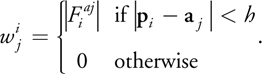
To accelerate the particle distribution process described in Section 7.3, we introduce a particle dispersion method. This method acts immediately on the position of the surface particles simulated by the GPU. We change the position of particles based on their particle density—defined in Equation 5—which can be calculated with the same nearest-neighbors algorithm used for calculation of repulsion forces. Particles from high-density areas are removed and placed at positions in areas with low density. To this end, we compare the densities of a base particle and a comparison particle to a certain threshold T. When the density of the comparison particle is lowest and the density difference is above the threshold, the position of the base particle will change in order to increase density at the comparison position and decrease it at the base position. The base particle will be moved to a random location on the edge of the influence area of the comparison particle, as shown in Figure 7-8, in order to minimize fluctuations in density at the position of the comparison particle. Such fluctuations would bring about even more particle relocations, which could make the fluid surface restless.

Figure 7-8 The Dispersion of Particles

It is infeasible to have every particle search the whole pool of surface particles for places of low density on the fluid surface at every iteration of the surface particle simulation. Therefore, for each particle, the GPU randomly selects a comparison particle in the pool every t seconds, by using a texture with random values generated on the CPU. The value of t can be chosen arbitrarily. Here is the algorithm:

For each surface particle:

Determine if it is time for the particle to switch position.
If so, choose the comparison position and compare densities at the two positions.
If the density at this particle is higher than the density at the comparison particle, with a difference larger than threshold T, change the position to a random location at the comparison particle's influence border.

To determine the threshold T, we use a heuristic, minimizing the difference in densities between the two original particle positions. This heuristic takes as input the particle positions p and q, with their densities before any position change _p0 and _q0 . It then determines if a position change of the particle originally at p increases the density difference between the input positions. The densities at the (fixed) positions p and q after the particle position change are _p1 and _q1 , respectively. Equation 9 is used by the heuristic to determine if there is a decrease in density difference after a position change, thereby yielding the decision for a change of position of the particle originally located at p.

Equation 9

Because the original particle would move to the edge of influence of the comparison particle—as you can see in Figure 7-8—the following equations hold in the case of a position change.

Equation 10

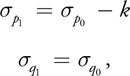
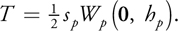
where k is the value at the center of the particle smoothing kernel, s _p W _p (0, h _p ). Using

Equation 9, substituting Equation 10, and solving for the initial density difference, we obtain Equation 11:

Equation 11

Equation 11 gives us the solution for our threshold T:

Equation 12

Still, it depends on the application of the dispersion algorithm if this threshold is enough to keep the fluid surface steady. Especially in cases where all particles can decide at the same time to change their positions, a higher threshold might be desired to keep the particles from changing too much. The effect of our particle distribution methods is visible in Figure 7-9. Both sides of the figure show a fluid simulation based on SPH, but in the sequence on the left, only particle repulsion is enabled, and on the right, both repulsion and dispersion are enabled. The particles sample a cylindrical fluid surface during a three-second period, starting from a bad initial distribution. Figure 7-9 shows that our particle dispersion mechanism improves upon the standard repulsion behavior considerably. We can even adapt the particle size based on the particle density, to fill gaps even faster. (You'll see proof of this later, in Figure 7-11.)

Figure 7-9 The Distribution Methods at Work: Surface Particles Spread over a Group of Fluid Atoms in the Form of a Cylinder

No matter how optimally the particle distribution algorithm performs, it can be aided by selecting reasonable starting locations for the particles. Because we do not know where the surface will be located for an arbitrary collection of fluid atoms, we try to guess the surface by positioning fluid particles on a sphere around every fluid atom. If we use enough surface particles, the initial distribution will make the surface look like a blobby object already. We assign an equal amount of surface particles to every fluid atom at the start of our simulation, and distribute them by using polar coordinates (r,) for every particle, varying and the z coordinate of r linearly over the number of surface particles assigned to a single atom.

Because particle dispersion acts on the positions of particles, we should query particle densities and change positions based on those densities during the position calculation pass in Figure 7-2. Listing 7-4 demonstrates a query on the repulsion force texture to obtain the surface particle density at a certain position.

Example 7-4. Excerpt from a Fragment Program Simulating the Position of a Surface Particle

 void mainpos(   . . .   in float4 particle : TEXCOORD0,   out float4 color : COLOR0,   const uniform float time_step,   const uniform samplerRECT rep_texture : TEXUNIT5,   const uniform float4x4 ModelViewProj) {   //ModelViewProj is the same as during repulsion calculation    //in Listing 7-3.    //oldpos and velocity passed through via textures    float3 newposition;   float  normalintegration = 1.0;   //Perform the query.   float4 transformedpos = mul(ModelViewProj, oldpos);   transformedpos /= transformedpos.w;   transformedpos.xy = transformedpos.xy * 0.5 + 0.5;   transformedpos.xy = float2(transformedpos.x * screen_width,                              transformedpos.y * screen_height);   float4 rep_density1 = texRECT(rep_texture, transformedpos.xy);   //1. If it's time to compare particles (determine via a texture or    //   uniform parameter)    //2. Make a query to obtain rep_density2 for another    //   particle (determine randomly via texture).    //3. If the density difference is greater than our threshold,    //   set newposition to edge of comparison particle boundary    //   (normalintegration becomes false).   if(normalintegration)     newposition = oldpos + velocity*time_step;   //Output the newposition.   color.xyz = newposition;   color.a = 1.0; }

7.5 Performance

The performance of our final application is influenced by many different factors. Figure 7-2 shows three stages that could create a bottleneck on the GPU: the particle repulsion stage, the constrained particle velocity calculation, and the particle dispersion algorithm. We have taken the scenario of water in a glass from Figure 7-11 in order to analyze the performance of the three different parts.

We found that most of the calculation time of our application was spent in two areas. The first of these bottlenecks is the calculation of constrained particle velocities. To constrain particle velocities, each particle has to iterate over a hash structure of fluid atom positions, performing multiple texture lookups and distance calculations at each iteration. To maximize performance, we have minimized the number of hash collisions by increasing the number of hash buckets. We have also chosen smaller grid cell sizes to decrease the number of redundant neighbors visited by a surface particle; the grid cell size is a third to a fifth of a fluid atom's diameter.

The second bottleneck is the calculation of the repulsion forces. The performance of the algorithm is mainly determined by the query size around a surface particle. A smaller size will result in less overdraw and faster performance. However, choosing a small query size may decrease particle repulsion too much. The ideal size will therefore depend on the requirements of the application. To give a rough impression of the actual number of frames per second our algorithm can obtain, we have run our application a number of times on a GeForce 6800, choosing different query sizes for 16,384 surface particles. The query sizes are visualized by quads, as shown in Figure 7-10.

Figure 7-10 Surface Particle Query Area Visualized for a Glass of Water, Using 16,384 Particles

7.6 Rendering

To demonstrate the level of realism achievable with our visualization method, Figure 7-11 shows examples of a fluid surface rendered with lighting, blending, surface normal curvature, and reflection and refraction. To render a smooth transparent surface, we have used a blending method that keeps only the frontmost particles and discards the particles behind others. The challenge lies in separating the particles on another part of the surface that should be discarded, from overlapping particles on the same part of the surface that should be kept for blending.

Figure 7-11 Per-Pixel Lit, Textured, and Blended Fluid Surfaces

To solve the problem of determining the frontmost particles, we perform a depth pass to render the particles as oriented quads, and calculate the projective-space position of the quad at every generated fragment. We store the minimum-depth fragment at every pixel in a depth texture. When rendering the fluid surface as oriented quads, we query the depth buffer only at the particle's position: the center of the quad. Using an offset equal to the fluid atom's radius, we determine if a particle can be considered frontmost or not. We render those particles that pass the test. This way, we allow multiple overlapping quads to be rendered at a single pixel.

We perform blending by first assigning an alpha value to every position on a quad, based on the distance to the center of the quad. We accumulate these alpha values in an alpha pass before the actual rendering takes place. During rendering, we can determine the contribution of a quad to the overall pixel color based on the alpha value of the fragment and the accumulated alpha value stored during the alpha pass.

Finally, we use a normal perturbation technique to increase detail and improve blending of the fluid surface. While rendering the surface as oriented quads, we perturb the normal at every fragment slightly. The normal perturbation is based on the curvature of the fluid density field at the particle position used for rendering the quad. The curvature of the density field can be calculated when we calculate the gradient and density field during the velocity constraint pass. Using the gradient, we can obtain a vector the size of our rendered quad, tangent to the fluid surface. This vector is multiplied by the curvature, a 3x3 matrix, to obtain the change in normal over the tangent vector. We only store the change in normal projected onto the tangent vector using a dot product, resulting in a scalar. This is the approximation of the divergence at the particle position (while in reality it constitutes only a part of the divergence). This scalar value is stored, and during surface rendering it is used together with the reconstructed tangent vector to form a perturbation vector for our quad's normal.

7.7 Conclusion

We have presented a solution for efficiently and effectively implementing the point-based implicit surface visualization method of Witkin and Heckbert 1994 on the GPU, to render metaballs while maintaining interactive frame rates. Our solution combines three components: calculating the constraint velocities, repulsion forces, and particle densities for achieving near-uniform particle distributions. The latter two components involve a novel algorithm for a GPU particle system in which particles influence each other. The last component of our solution also enhances the original method by accelerating the distribution of particles on the fluid surface and enabling distribution among disconnected surfaces in order to prevent gaps. Our solution has a clear performance advantage compared to marching cubes and ray-tracing methods, as its complexity depends on the fluid surface area, whereas the other two methods have a complexity depending on the fluid volume.

Still, not all problems have been solved by the presented method. Future adaptations of the algorithm could involve adaptive particle sizes, in order to fill temporarily originating gaps in the fluid surface more quickly. Also, newly created disconnected surface components do not always have particles on their surface, which means they are not likely to receive any as long as they remain disconnected. The biggest problem, however, lies in dealing with small parts of fluid that are located far apart. Because the repulsion algorithm requires a clip space encapsulating every particle, the limited resolution of the viewport will likely cause multiple particles to map to the same pixel, implying data loss. A final research direction involves rendering the surface particles to achieve various visual effects, of which Figure 7-11 is an example.

7.8 References

Blinn, James F. 1982. "A Generalization of Algebraic Surface Drawing." In ACM Transactions on Graphics 1(3), pp. 235–256.

Latta, Lutz. 2004. "Building a Million Particle System." Presentation at Game Developers Conference 2004. Available online at http://www.2ld.de/gdc2004/.

Lorensen, William E., and Harvey E. Cline. 1987. "Marching Cubes: A High Resolution 3D Surface Construction Algorithm." In Proceedings of the 14th Annual Conference on Computer Graphics and Interactive Techniques, pp. 163–169.

Müller, Matthias, David Charypar, and Markus Gross. 2003. "Particle-Based Fluid Simulation for Interactive Applications." In Proceedings of the 2003 ACM SIGGRAPH/Eurographics Symposium on Computer Animation, pp. 154–159.

Parker, Steven, Peter Shirley, Yarden Livnat, Charles Hansen, and Peter-Pike Sloan. 1998. "Interactive Ray Tracing for Isosurface Rendering." In Proceedings of the Conference on Visualization'98, pp. 233–238.

Pascucci, V. 2004. "Isosurface Computation Made Simple: Hardware Acceleration, Adaptive Refinement and Tetrahedral Stripping." In Proceedings of Joint EUROGRAPHICS3—IEEE TCVG Symposium on Visualization 2004.

Teschner, M., B. Heidelberger, M. Mueller, D. Pomeranets, and M. Gross. 2003. "Optimized Spatial Hashing for Collision Detection of Deformable Objects." In Proceedings of Vision, Modeling, Visualization 2003.

Vrolijk, Benjamin, Charl P. Botha, and Frits H. Post. 2004. "Fast Time-Dependent Isosurface Extraction and Rendering." In Proceedings of the 20th Spring Conference on Computer Graphics, pp. 45–54.

Witkin, Andrew P., and Paul S. Heckbert. 1994. "Using Particles to Sample and Control Implicit Surfaces." In Proceedings of the 21st Annual Conference on Computer Graphics and Interactive Techniques, pp. 269–277.

Part II: Light and Shadows

Part III: Rendering

Part IV: Image Effects

Part V: Physics Simulation

Part VI: GPU Computing

Preface