GPU Gems 3

GPU Gems 3 is now available for free online!

The CD content, including demos and content, is available on the web and for download.

You can also subscribe to our Developer News Feed to get notifications of new material on the site.

Chapter 4. Next-Generation SpeedTree Rendering

Alexander Kharlamov
NVIDIA Corporation

Iain Cantlay
NVIDIA Corporation

Yury Stepanenko
NVIDIA Corporation

4.1 Introduction

SpeedTree is a middleware package from IDV Inc. for rendering real-time trees. A game that uses SpeedTree has great flexibility in choosing how to render SpeedTrees. We discuss several features of the GeForce 8800 that enable high-quality, next-generation extensions to SpeedTree. First, silhouette clipping adds detail to branch and trunk outlines. Next, shadow mapping adds realistic self-shadowing at the level of individual leaves. Additionally, we further refine the lighting with a two-sided-leaf lighting model and high-dynamic-range (HDR) rendering. Finally, multisample antialiasing along with alpha to coverage provide very high visual quality, free from aliasing artifacts.

4.2 Silhouette Clipping

Tree branches and trunks are organic, irregular, and complex. Figure 4-1 shows a typical, real example: although the branches are approximately cylindrical, the detailed silhouette is rough and irregular. A medium-polygon or low-polygon tree trunk mesh, say 1,000 polygons, cannot capture this detail. The resulting straight polygonal edges are a subtle but important cue that you are seeing a computer-generated image.

Figure 4-1 A Photograph of a Real Tree Branch, with an Irregular Silhouette

Many algorithms are available to help represent the large amount of detail seen in the branch depicted in Figure 4-1. The oldest and most widely implemented of these techniques is bump mapping. Bump mapping provides a reasonably good representation of the interior region of the branch, such as the region within the lime square in Figure 4-1. However, it is completely unable to handle the details of the silhouette highlighted in the blue squares. It also fails to handle the parallax a viewer should observe from the varying depth of the bark. Improving on bump mapping are a pair of related techniques: relief mapping (Oliveira and Policarpo 2005) and parallax occlusion mapping (POM)(Tatarchuk 2006). Both techniques perform shallow ray tracing along the surface of the object, which can add parallax and self-occlusion. (We use relief mapping as the generic term to cover both.) With parallax occlusion mapping, the effect is again limited to the interior of the object, and the silhouette is unchanged. Relief mapping offers several extensions, one of which supports silhouettes, but it requires additional preprocessing to enable it. Finally, tessellation of the model and displacement mapping can also be used, but they create a significant overhead in geometry processing that may not be worthwhile when trying to render a whole forest full of trees.

Our approach is to utilize relief mapping on the trunks of the trees to handle the interior detail, and to perform an additional pass to provide silhouette details. None of this is supported by the SpeedTree reference shaders, but they can be easily added because the tools, file format, and API allow for additional custom functionality, including extra texture maps.

For the silhouettes, we employ a technique that we call silhouette clipping. Although the technique differs significantly from the original described in Sander et al. 2000, the net effect is very similar. Our technique extrudes fins from the silhouette of the object in a direction perpendicular to the view vector. These silhouettes undergo a ray tracing of the height map similar to relief mapping to determine which pixels should actually be occluded by the silhouette. As with the relief mapping used on the branch polygons, this technique requires no additional preprocessing work.

4.2.1 Silhouette Fin Extrusion

The first step in rendering the silhouettes is to extrude the fins. We do this by using smooth, per-vertex normals to determine the silhouette edge within a triangle. If the dot product of the vertex normal and the view vector changes sign along a triangle edge, then we find a new vertex on that edge, in the position where the dot product of the interpolated view vector and interpolated normal equals zero. Figure 4-2 illustrates the procedure.

Figure 4-2 Side View of Silhouette Extrusion on a Single Triangle

Finding silhouettes and fin extrusion can be performed directly on DirectX 10 hardware. We calculate the dot product between the vertex normals and view vector inside the vertex shader. After that, the geometry shader compares the signs of the dot products and builds two triangles at the points where the dot product equals zero, as shown in Figure 4-2c and Figure 4-2d. Because the two triangles are generated as a strip, the maximum number of vertices output from the geometry shader output is four. If the dot product sign does not change within the triangle, the geometry shader does not output anything. If a single vertex normal turns out to be orthogonal to the view vector, then our calculations will produce a degenerate triangle. Naturally, we do not want to waste time processing such triangles, so we check for this case, and if we find that two of the triangle's positions are the same, we do not emit this triangle from the geometry shader. Figure 4-3 shows an example of the intermediate output.

Figure 4-3 Tree Trunks with Silhouette Fins (in Wireframe)

To ensure continuity along the silhouette, the algorithm requires smooth, per-vertex, geometric normals. This requirement conflicts with SpeedTree's optional "light-seam reduction" technique, whereby branch normals are bent away from the geometric normal to avoid lighting discontinuities. To support both features, two different normals have to be added to the vertex attributes.

4.2.2 Height Tracing

Once the fins have been extruded, we use a height map to present a detailed object silhouette. The height map is the same one used by the main trunk mesh triangles for relief mapping, but silhouette fins need a more sophisticated height map tracing algorithm. We extrude additional geometry from vertices V ₀ and V ₁, as shown in Figure 4-4. For this fin we will need the following:

The tangent basis, to calculate diffuse lighting
The vertex position, to shadow fins correctly
The texture coordinates
The view vector, for height tracing

Figure 4-4 Vertex Attributes for Extruded Geometry

There is no need to calculate new values for tangent basis and texture coordinates, for vertexes V ₂ and V ₃. V ₂ attributes are equal to V ₁ attributes, whereas V ₃ attributes are equal to V ₀ attributes, even though that is theoretically incorrect.

Figure 4-5 demonstrates how this works. It shows that we compute a different view vector for every vertex. In the pixel shader, we first alter the texture coordinate from the fin (point A) by making a step backward in the direction of the view vector (the view vector is in tangent space after the geometry shader). We clamp the distance along the view vector to be no more then an experimentally found value and we arrive at point B. It is possible that point B can be different for different fragments. After that, we perform the usual relief-mapping height-tracing search. If we find an intersection, then we calculate diffuse illumination and shadowing for this fragment. Otherwise, the fragment is antialiased (see Section 4.6.3) or discarded.

Figure 4-5 Height Tracing Along the View Vector

For silhouette fins, the search through the height map will trace along a longer footprint in texture space because, by definition, the view vector intersects the mesh at a sharp angle at the silhouette. Thus, the fins require more linear search steps than the relief mapping on the main trunk polygons. Fortunately, the fins are always small in terms of shaded screen pixels, and as a result, the per-pixel costs are not significant. We also clamp the length of the search in texture space to a maximum value to further limit the cost. Figure 4-6 shows a cylinder with attached fins. It illustrates how the fins are extruded from simple geometry. Figure 4-7 shows the same cylinder, textured. Relief mapping combined with silhouettes show realistic, convincing visual results.

Figure 4-6 Wireframe with Silhouette Fins

Figure 4-7 The Result of Relief Mapping and Height Tracing

Although the algorithm presented here produces excellent results, in many ways it is simply the tip of the iceberg. We rely on simple linear height map tracing for relief mapping. This can be improved by using a combination of linear and binary searches as in Policarpo 2004 or using additional precomputed data to speed up the tracing algorithm (Dummer 2006, Donnelly 2005). Additionally, self-shadowing can be computed by tracing additional rays.

4.2.3 Silhouette Level of Detail

Even with the optimizations, note that silhouettes are not required for most trees. At distance, silhouettes' visual impact is insignificant. Because they do require significant pixel and geometry cycles, we remove them from distant trees. For each tree type, there is a transition zone during which the width of the silhouettes, in world coordinates, is gradually decreased to zero as a function of distance, as shown in Figure 4-8. Thus they don't pop when they are removed. In practice, the number of visible silhouettes is limited to less than ten in typical scenes, such as those appearing in Section 4.7.

Figure 4-8 The Silhouette Falloff Function

4.3 Shadows

With the tree silhouettes improved, we move on to raise the quality of the shadows. Because general shadow techniques are specific to each game engine, out-of-the-box SpeedTree shadows are precomputed offline and static—a lowest-common-denominator approach so that SpeedTree can work with many different engines. This approach has some drawbacks:

When the tree model animates due to the wind effect, shadow animation is limited to transformations of the texture coordinates: stretching, rotation, and so on.
Precomputed shadows don't look as realistic as dynamic ones, especially shadows projected onto the tree trunks.
The leaves do not self-shadow.

4.3.1 Leaf Self-Shadowing

Our second major goal is to make the leaves look individually shadowed within the leaf card. (SpeedTree uses both flat leaf cards and 3D leaf meshes; this section details leaf card self-shadowing.) Leaf self-shadowing is not straightforward, because leaf cards are simplified, 2D representations of complex 3D geometry. The leaf cards always turn to face the camera, and as a result, they are all parallel to the view plane. Figure 4-9 shows a tree with leaf cards. In this method, we use shadow mapping. (See King 2004 for an introduction to shadow-mapping techniques.) To make the shadows look visually appealing, we have altered both the process of generating the shadow map and the technique of shadow-map projection.

Figure 4-9 A Shadow Map Projected Vertically onto Leaf Cards

Our generation of shadow maps for leaves largely follows standard rendering. Leaf cards turn to face the view position. When rendering to the shadow map, they turn to face the light source and thus make good shadow casters. However, as Figure 4-10 illustrates, they rotate around their center point, which presents a problem. In the figure, the pale blue leaf card is rotated toward the viewer; the lime leaf card represents the same leaf card, but now rotated toward the light source. In Figure 4-10a, note that the lime leaf card will shadow only the lower half of the blue leaf card during the shadow projection. To avoid this artifact, we simply translate the lime leaf card toward the light source, as shown in Figure 4-10b. We translate it by an arbitrary, adjustable amount, equal to approximately half the height of the leaf card.

Figure 4-10 Leaf Card Positioning

The planar geometry of leaf cards poses a more significant problem when applying the shadow map. Applying a shadow map to a planar leaf card will result in the shadows being projected along the 2D leaf card as elongated streaks (see Figure 4-12). The only case that works well is a light source near the eye point.

To shadow leaf cards more realistically, without streaks, during the shadow application pass, we alter the shadowed position by shifting it in the view direction. (Note that we are not altering the geometric, rasterized position—the leaf card is still a 2D rectangle. We only shift the position used for the shadowing calculation.) The offset coefficient is stored in a texture and is uniform across each individual leaf inside the leaf card. Figure 4-11 shows the resulting texture. Using this new leaf position, we project the shadowed pixel into light space and sample the shadow map. Because this operation alters different leaves inside the leaf card independently, it has to be performed in a pixel shader. The function used for performing these operations is detailed in Listing 4-1.

Figure 4-11 Leaf Texture and Accompanying Depth-Offset Texture

Example 4-1. Pixel Shader Code to Apply Shadow Maps with Offsets

    float PSShadowMapFetch(Input In) {   // Let In.VP and In.VV be float3;   // In.VP - interpolated Vertex Position output by VS   // In.VV - View Vector output by VS   // OCT - Offset Coefficient Texture   // SMPP - Shadow Map Pixel Position   // SMMatrix - transform to Shadow Map space   float3 SMPP = In.VP + In.VV * tex2D(OCT, In.TexCoord).x;   float3 SMCoord = mul(SMMatrix, float4(SMPP, 1));   float SM = tex2D(SMTexture, SMCoord);   return SM; }

Figure 4-12 shows the results of both types of offset. (Except for the shadow term, all other lighting and color has been removed to emphasize the shadow.) Two types of artifacts are visible in the Figure 4-12a: there are vertical streaks due to the projection of the shadow map vertically down the 2D leaf cards. There are also diagonal lines at the positions of the leaf cards when the shadow map is rendered. In Figure 4-12b, these artifacts are eliminated. The result is very detailed and natural foliage. In our real-time demo, the self-shadowing of individual leaves varies as the tree moves due to wind.

Figure 4-12 The Impact of Leaf Offsets with Self-Shadowing

4.3.2 Cascaded Shadow Mapping

Improving the shadowing behavior of the tree leaves unfortunately does not free the scene from other shadow-map artifacts. For vast outdoor scenes, a single shadow map is usually insufficient. Cascaded shadow mapping (CSM) is a common technique that addresses this problem by splitting the view frustum into several areas and rendering a separate shadow map for each region into different textures. (A description of CSM can be found in Zhang et al. 2006. Also, see Chapter 10 of this book, "Parallel-Split Shadow Maps on Programmable GPUs," for more on shadow maps and a technique that is related to CSM.)

To reduce CPU overhead, different cascades are updated with different frequencies:

The closest cascade is updated every frame. All objects are rendered into it.
The second cascade is updated every two frames. Fronds are not rendered into the shadow map.
The third cascade is updated every four frames. Only leaves are rendered into the shadow map.

After the shadow maps are rendered, we have many ways to actually shadow our 3D world:

Render objects in the same order as they were rendered during shadow-map rendering, using an appropriate cascade.
Fetch pixels from every cascade and mix them.
Use texture arrays and choose the appropriate cascade in the pixel shader.
Split one render target into several shadow maps, using viewports.

Every approach has its own pros and cons. In SpeedTree, we chose the second option.

4.4 Leaf Lighting

Lighting plays an important role in viewers' perception. The latest versions of SpeedTree provide all the data necessary to perform per-pixel dynamic lighting on the leaf cards, including tangents and normal maps. Alternatively, leaf cards in SpeedTree can use precomputed textures with diffuse lighting only. Detailed lighting and shadows are prebaked into the diffuse textures. We have opted for the first solution, because it supports a fully dynamic lighting environment.

4.4.1 Two-Sided Lighting

In addition to the differences in specular lighting, we observed that leaves look different depending on the view's position relative to the light. Figure 4-13 shows two photographs of the same leaves taken seconds apart, in the same lighting conditions, with the same camera settings for exposure, and so on. (Look closely at the brown spots of disease and you can compare the same leaf in both photos. One leaf is marked by a red spot.) When a leaf is lit from behind, the major contribution is not reflected light; instead, the major contribution to the illumination is from transmitted light. As the light shines through the leaf, its hue is slightly shifted to yellow or red.

Figure 4-13 Real Leaf Lighting as a Function of View Direction

Based on this observation, we have implemented the following scheme to simulate the two-sided nature of the illumination:

Yellow leaf color is generated inside the pixel shader as a float3 vector with components (Diffuse.g * 0.9, Diffuse.g * 1.0, Diffuse.g * 0.2).
Depending on the value of µ - angle, as shown in Figure 4-14, between light direction and view vector, we lerp between the original color and the yellow version. Lerping occurs if µ is close to , which means that we are looking at the sun, and if the tree is in our way, leaves will appear slightly more yellow.

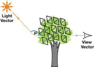
Figure 4-14 Back-Lighting of Leaves

Depending on µ, the specular component is reduced, because no light reflection should occur on the back side. This approach may seem naive, but it makes the picture more visually appealing. See Figure 4-15.

Figure 4-15 Lighting Enhancement Comparison

4.4.2 Specular Lighting

In addition to the tweaks for two-sided lighting, we modify the specular illumination to enhance the realism. First, with normal specular lighting, distant trees tend to shimmer, so we reduce specular lighting according to distance. Next, we observed actual tree leaves to get some additional clues. Figure 4-16 shows some typical shiny leaves, and from it we observe three points. The specular reflection is dominated by a strong division of the leaf into two planes along its axis. Relative to the effect of these planes, the fine detail of the veins and other features is fairly insignificant. The specular power of the reflection is low: the reflections are not sharp, as they are on, say, a glassy material. Because we are interested in modeling on the scale of whole trees, not leaf veins, we use these observations to simplify our leaf specular model. To simulate the axial separation, we use a coarser V-shaped normal map to split the leaf into two halves. Finally, because too much detail in the specular contribution often results in shimmering, we bias the texture fetch to a lower mipmap level of the normal map. The end result is smoother, gentler specular lighting that does not introduce heavy lighting-related aliasing.

Figure 4-16 A Photograph of Leaves, Showing the Behavior of Specular Illumination

4.5 High Dynamic Range and Antialiasing

Our SpeedTree demo implements high dynamic range combined with multisample antialiasing (MSAA). We use a GL_RGBA16F_ARB format frame buffer, in conjunction with the GL_ARB_multisample extension.

High-range frame-buffer values come from the sky box, which is an HDR image, and from the tree rendering. SpeedTree supports overbright rendering. Our demo adjusts this so that it outputs values ever so slightly outside the [0, 1] range.

A post-processing filter adds "God rays" to bright spots in the frame buffer by using a radial blur. Otherwise, our use of HDR is not new.

4.6 Alpha to Coverage

Alpha to coverage converts the alpha value output by the pixel shader to a coverage mask that is applied at the subpixel resolution of an MSAA render target. When the MSAA resolve is applied, the result is a transparent pixel. Alpha to coverage works well for antialiasing what would otherwise be 1-bit transparency cutouts.

4.6.1 Alpha to Coverage Applied to SpeedTrees

Such 1-bit cutouts are common in rendering vegetation, and SpeedTree uses transparent textures for fronds and leaves. We apply alpha to coverage to these textures, and Figure 4-17 shows the benefits when applied to fronds. The pixelation and hard edges in the left-hand image are greatly reduced when alpha to coverage is applied. The benefits are greater when the vegetation animates (SpeedTree supports realistic wind effects), as the harsh edges of transparency cutouts tend to scintillate. Alpha to coverage largely eliminates these scintillation artifacts. Unlike alpha blending, alpha to coverage is order independent, so leaves and fronds do not need to be sorted by depth to achieve a correct image.

Figure 4-17 The Impact of Alpha to Coverage

4.6.2 Level-of-Detail Cross-Fading

However, there is a problem. The reference SpeedTree renderer uses alpha cutouts for a different purpose: fizzle level of detail (LOD). A noise texture in the alpha channel is applied with a varying alpha-test reference value. As the reference value changes, differing amounts of the noise texture pass the alpha test. (For more details, see Whatley 2005.)

To cross-fade between LODs, two LOD models are drawn simultaneously with differing alpha-test reference values. The fizzle uses alpha test to produce a cross-fade at the pixel level. All sorts of things went wrong when alpha to coverage was naively applied in conjunction with fizzle LOD (most obviously, the tree trunks became partly transparent).

Fortunately, alpha to coverage can also be adapted to implement the cross-fade. Alpha to coverage is not a direct replacement for alpha blending: large semitransparent areas do not always work well. In particular, alpha to coverage does not accumulate in the same way as blended alpha. If two objects are drawn one on top of the other with 50 percent alpha-to-coverage alpha, they both use the same coverage mask. The resulting image is the object that passes the depth test, drawn with 50 percent transparency.

We solve this problem by offsetting the alpha-fade curves of the two LODs. The result is not perfect: at some points during a transition, the overall tree is still more transparent than we would like. But this defect is rarely noticeable in practice. Figure 4-18 shows a tree in the middle of a cross-fade, using alpha to coverage.

Figure 4-18 A Tree in the Middle of an LOD Cross-fade

4.6.3 Silhouette Edge Antialiasing

In our silhouette-clipping algorithm, height tracing is performed in the pixel shader. This means that the silhouette outline is determined only for each pixel, not for each sample. Because the visible edge is no longer the geometric edge, standard multi-sampling does not antialias the visible edge.

Alpha to coverage can be used to antialias the silhouette edges. To do this, we generate a narrow border region, at the edge of the silhouette, across which the silhouette opacity fades from opaque to clear.

We store 1 or 0 in the view vector W component in the geometry shader. Vertices V ₀ and V ₁ store 0 and V ₂ and V ₃ store 1, as shown in Figure 4-19. This value will be interpolated across the fin and represent a smooth height change.

Figure 4-19 The Alpha Distribution on a Silhouette Fin

During height tracing, we remember the minimal miss against the height map and change the pixel opacity according to that value. We take ddx() and ddy() of the view vector's W component to determine height change per pixel. After that, we check the minimal miss (from view vector to height map tracing) against the footprint to determine pixel alpha as a linear function. The alpha value equals 1.0 if the view vector intersects the trunk height map. If we miss, we let alpha fade to 0 if the minimal miss is less than about 1.5 pixels in screen-space units. Otherwise, alpha is set to 0.

Figure 4-20 shows a silhouette without antialiasing and the same silhouette with our alpha-to-coverage border applied.

Figure 4-20 Alpha-to-Coverage Antialiasing on Extruded Silhouettes

4.7 Conclusion

The figures in this final section show some typical results obtained using our techniques. They bring all of our GeForce 8800 SpeedTree techniques together in a high-quality demo. Figure 4-21 shows our two-sided leaf-lighting model interacting with high-dynamic-range effects. Detailed trunk silhouettes are also clearly visible. Close inspection of the trunk near the bottom center of Figure 4-21 shows some discontinuity artifacts between the trunk mesh and the silhouette. However, we find these artifacts small and acceptable.

Figure 4-21 Two-Sided Leaf Lighting and Branch Silhouettes

Figure 4-22 demonstrates silhouette clipping applied to a quite different trunk type: the tall, thin trees. Note how the silhouette bumps correspond well with the relief-mapped bumps applied to the trunk mesh. The silhouettes also have a subtle effect on the thinnest trunks, for example, on the very right edge of the image. The effect is subtle, but it breaks up what are otherwise straight polygonal edges. Lighting and HDR effects are also visible, and all the trees show detailed self-shadowing.

Figure 4-22 High Dynamic Range and Two-Sided Lighting Plus Silhouettes

Figure 4-23 shows a closer view of our shadowing. The foreground tree casts accurate shadows on the rock below and on its own trunk, including the silhouette fins. These shadows move realistically as the tree sways due to SpeedTree's wind effects. The leaves in the very top right and in the center of the image demonstrate self-shadowing. This depiction is not strictly accurate, but it is realistic. The light source is almost directly overhead. Note how the shadowing of the leaves reflects this: in the center of the image, the clusters are lit at the top and in shadow at the bottom, with a realistic dappling in between.

Figure 4-23 Detailed, Accurate Self-Shadowing

Note also the effect of the cascaded shadow maps. A highly detailed shadow is visible in the foreground of Figure 4-23. Yet, just to the right of the center, shadows are cast by distant trees, to the limit of the view distance. All visible shadows are dynamically generated and move as the trees animate.

These images demonstrate that SpeedTree's shaders can be readily customized well beyond the standard reference implementation. They also demonstrate that the NVIDIA GeForce 8800 is capable of rendering extremely high quality, realistic vegetation.

4.8 References

Donnelly, William. 2005. "Per-Pixel Displacement Mapping with Distance Functions." In GPU Gems 2, edited by Matt Pharr, pp. 123–136. Addison-Wesley.

Dummer, Jonathan. 2006. "Cone Step Mapping: An Iterative Ray-Heightfield Intersection Algorithm." Available online at http://www.lonesock.net/files/ConeStepMapping.pdf.

King, Gary. 2004. "Shadow Mapping Algorithms." Presentation. Available online at ftp://download.nvidia.com/developer/presentations/2004/GPU_Jackpot/ Shadow_Mapping.pdf.

Lloyd, Brandon, David Tuft, Sung-Eui Yoon, and Dinesh Manocha. 2006. "Warping and Partitioning for Low Error Shadow Maps." In Proceedings of the Eurographics Symposium on Rendering 2006, pp. 215–226.

NVIDIA Corporation. 2005. "Anti-Aliasing with Transparency." White paper. Available online at http://http.download.nvidia.com/developer/SDK/Individual_Samples/DEMOS/Direct3D9/src/AntiAliasingWithTransparency/docs/AntiAliasingWithTransparency.pdf.

Oliveira, Manuel, Gary Bishop, and David McAllister. 2000. "Relief Texture Mapping." In ACM Transactions on Graphics (Proceedings of SIGGRAPH 2000) 19(3), pp. 359–368.

Oliveira, Manuel, and Fabio Policarpo. 2005. "An Efficient Representation for Surface Details." UFRGS Technical Report RP-351. Available online at http://www.inf.ufrgs.br/~oliveira/pubs_files/Oliveira_Policarpo_RP-351_Jan_2005.pdf.

Policarpo, Fabio. 2004. "Relief Mapping in a Pixel Shader Using Binary Search."

Sander, Pedro, Xianfeng Gu, Steven Gortler, Hugues Hoppe, and John Snyder. 2000. "Silhouette Clipping." In ACM Transactions on Graphics (Proceedings of SIGGRAPH 2000) 19(3), pp. 327–334.

Tatarchuk, N. 2006. "Dynamic Parallax Occlusion Mapping with Approximate Soft Shadows." In Proceedings of ACM SIGGRAPH Symposium on Interactive 3D Graphics and Games 2006, pp. 63–69.

Whatley, David. 2005. "Toward Photorealism in Virtual Botany." In GPU Gems 2, edited by Matt Pharr, pp. 7–26. Addison-Wesley.

Zhang, F., H. Sun, L. Xu, and K. L. Lee. 2006. "Parallel-Split Shadow Maps for Large-Scale Virtual Environments." In Proceedings of ACM International Conference on Virtual Reality Continuum and Its Applications 2006, pp. 311–318.

Part II: Light and Shadows

Part III: Rendering

Part IV: Image Effects

Part V: Physics Simulation

Part VI: GPU Computing

Preface