Ray tracing is a rendering algorithm that can generate photorealistic images by simulating how light transmits and interacts with different materials. Today, it is widely adopted to bring imagery to life in game development, film-making, and physics simulations.
However, the ray-tracing algorithm is computationally intensive and requires hardware acceleration on the GPU to achieve real-time performance.
To leverage the hardware power for ray tracing, various toolchains and languages were invented to suit the need, such as openGL and the shading language.
Often, the build process of these software toolchains poses significant challenges to Python developers. To alleviate the difficulty and provide a familiar environment for writing ray tracing kernels, NVIDIA developed the Numba extension for PyOptiX. This extension enables graphics researchers and application developers to reduce the time from idea to implementation and shorten the development cycle on each iteration.
In this post, I provide an overview of the NVIDIA ray-tracing engine PyOptiX and explain how the Python JIT compiler, Numba, accelerates Python code. Finally, with a complete ray tracing example, I walk you through the steps of using the Numba extension for PyOptiX and write an accelerated ray tracing kernel in Python.
What are NVIDIA OptiX and PyOptiX?
NVIDIA RTX technology made ray tracing the default rendering algorithm in many modern rendering pipelines. As the demand for unique looks is unlimited, there’s a need for flexibility in customizing the rendering pipeline.
The NVIDIA RTX ray-tracing pipeline is customizable. By configuring how light transmits, reflects, and refracts on various materials, you can achieve distinctive looks on objects, such as shiny, glossy, or semi-transparent. By configuring how light rays are generated, you change the field of view and perspective of the look accordingly.
To address this need, NVIDIA developed NVIDIA OptiX, a ray-tracing engine that enables you to configure a hardware-accelerated ray-tracing pipeline. PyOptiX is the NVIDIA OptiX Python interface. This interface offers the capability for Python developers to have the same capabilities as NVIDIA OptiX developers who write in C++.
Kernel functions
To customize image facets, you use kernel functions, also referred to as kernel methods or kernels. You can think of kernels as a group of algorithms that transform data inputs to the required form. Native NVIDIA OptiX developers can write kernels with CUDA. With a Numba extension, you can write ray-tracing kernels in Python.
Higher performance with Numba and Numba.cuda
Ray tracing is a compute-intensive algorithm. While it is theoretically possible to run the ray-tracing kernel with the standard CPython interpreter, it would take days to render a regular ray-traced image. Moreover, NVIDIA OptiX requires the kernel to be runnable on a GPU device so that it integrates with the rest of the rendering pipeline.
Using Numba, a just-in-time Python function compiler, you can execute and accelerate your Python ray-tracing kernels with GPU hardware. Numba parses the Python function code and converts it to efficient machine code. On a high level, this process is divided into seven steps:
- The function’s byte code is generated with the bytecode compiler.
- The bytecode is analyzed. The control flow graph (CFG) and the data flow graph (DFG) are generated.
- With bytecode, CFG, and DFG, the Numba intermediate representation (IR) is generated.
- Based on the type of function inputs, the type is inferred for each IR variable.
- The Numba IR is rewritten and gets Python-specific optimization.
- The Numba IR is lowered to the LLVM IR, and more general optimization is performed.
- The LLVM IR is consumed by the LLVM backend and optimized GPU machine code is generated.
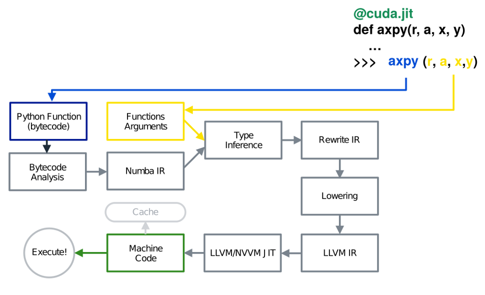
Figure 1 shows a graphical overview of the previously mentioned compilation pipeline. This quick tour of Numba’s compiler pipeline only provides a glimpse over Numba’s internal architecture. For more information, see The Life of a Numba Kernel: A Compilation Pipeline Taking User Defined Functions in Python to CUDA Kernels.
The following code shows an example GPU kernel that computes the dot product of two 3-element vectors.
@cuda.jit(device=True)
def dot(a, b):
   return a.x * b.x + a.y * b.y + a.z * b.z
Because Numba can convert any Python functions into native code, in a Numba CUDA kernel, Python users have equal power as if they are writing the kernel in native CUDA. This code shows a dot product that’s executable on the device. For more information, see Numba Examples.
Introducing the Numba extension for PyOptiX
To customize specific stages of the ray-tracing pipeline, you must translate the Numba kernel into something that can be understood by the NVIDIA OptiX engine. NVIDIA developed the Numba Extension for PyOptiX to achieve this goal.
The extension includes custom type definition and intrinsic function lowerings. NVIDIA OptiX comes with a set of internal types:
OptixTraversableHandleOptixVisibilityMaskSbtDataPointer- Functions such as
optix.Trace
For Numba to perform type inference on these new types and methods, you must register these types and provide an implementation of these methods before compiling the user kernel. Currently, NVIDIA is expanding supported types and intrinsics to add more examples.
By exposing these types and intrinsics to Numba, you can now write kernels, which not only target the GPU but can specifically target the GPU for ray-tracing kernels. In combination with Numba CUDA, you can write ray-tracing kernels of equal power as if you were writing native CUDA ray-tracing kernels for NVIDIA OptiX.
In the next section, I introduce a Hello World example with the PyOptiX Numba extension. Before that, let me quickly go over some ray-tracing algorithm basics.
Fundamentals of ray tracing
Imagine that you use a camera to capture an image. The light source in the scene emits light rays, which travel in a straight line. When a light ray hits an object, it is reflected from the surface and eventually reaches the camera sensor.
From a high level, a ray-tracing algorithm walks through all rays that reach the image plane to identify in the scene where and what the ray intersects with. When the intersection point is found, you can adopt various shading techniques to determine the color of the intersected point. However, there are also rays that don’t hit anything in the scene. In this case, these rays are considered as “missing” the target.
Steps for ray tracing a triangle with the Numba extension for PyOptiX
In the following example, I show how the Numba extension for PyOptiX can help you write custom kernels to define the ray behavior at ray generation, ray hit, and ray miss.
Scene setup
I modeled the view you see as an image plane, which usually sits slightly in front of the camera. The camera is modeled as a point and a set of mutually orthogonal vectors in the 3D space.
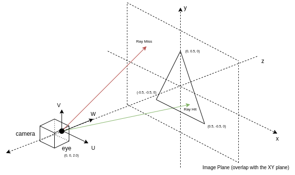
Camera
The camera is modeled as a point in three dimensions. The three vectors, U, V, and W, are used to show the sideways, upwards, and frontal directions of the camera. This uniquely determines the position and orientation of the camera.
To simplify the computation for ray generation later, the U and V vectors are not unit vectors. Instead, their lengths proportionally match the image’s aspect ratio. Lastly, the length of the W vector is the distance between the camera and the image plane.
Ray generation kernel
The ray generation kernel is the centerpiece of the algorithm. Ray origins and directions are generated here and then passed down to the trace call. Its intensity is retrieved from other kernels and written as image data. In this section, I discuss the methods used to generate rays in this kernel.
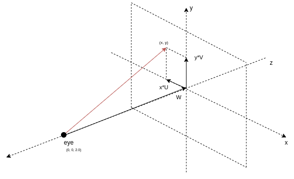
With the camera and the image plane, you can generate the rays. Adopt a coordinate system convention where the center of the image is the origin. The sign of a coordinate in an image pixel shows its relative position to the origin and its magnitude shows the distance. With this property, multiply the camera’s U and V vector with the corresponding elements of the pixel position and add them together. The result is a vector that points to the pixel from the image center.
Finally, add this vector to the W or front vector, and this generates a ray that originates at the camera position and goes through the pixel on the image plane. Figure 3 shows the decomposition of a ray that originates from the camera and goes through point (x, y) in the image plane.
In code, the pixel index and image dimension of the image plane can be retrieved using two optix intrinsic functions optix.GetLaunchIndex and optix.GetLaunchDimensions. Next, the pixel index is normalized to [-1.0, 1.0]. The following code example shows this logic in the Numba CUDA kernel.
@cuda.jit(device=True, fast_math=True)
def computeRay(idx, dim):
   U = params.cam_u
   V = params.cam_v
   W = params.cam_w
   # Normalizing coordinates to [-1.0, 1.0]
   d = float32(2.0) * make_float2(
       float32(idx.x) / float32(dim.x), float32(idx.y) / float32(dim.y)
   ) - float32(1.0)

   origin = params.cam_eye
   direction = normalize(d.x * U + d.y * V + W)
   return origin, direction

def __raygen__rg():
   # Look up your location within the launch grid
   idx = optix.GetLaunchIndex()
   dim = optix.GetLaunchDimensions()

   # Map your launch idx to a screen location and create a ray from the camera
   # location through the screen
   ray_origin, ray_direction = computeRay(make_uint3(idx.x, idx.y, 0), dim)
This code example shows the helper function of computeRay that computes the origin and direction vector of the ray.
Next, pass the generated ray into the intrinsic function optix.Trace. This initializes the ray tracing algorithm. The underlying optiX engine traverses through the primitives, computes the intersection point in the scene, and finally returns the intensity of the ray. The following code example shows the call to optix.Trace.
# In __raygen__rg
   payload_pack = optix.Trace(
       params.handle,
       ray_origin,
       ray_direction,
       float32(0.0),  # Min intersection distance
       float32(1e16), # Max intersection distance
       float32(0.0),  # rayTime -- used for motion blur
       OptixVisibilityMask(255),  # Specify always visible
       uint32(OPTIX_RAY_FLAG_NONE),
       uint32(0),  # SBT offset   -- Refer to OptiX Manual for SBT
       uint32(1),  # SBT stride   -- Refer to OptiX Manual for SBT
       uint32(0),  # missSBTIndex -- Refer to OptiX Manual for SBT
   )
Ray hit kernel
In the ray hit kernel, you write code to determine the intensity of each channel of the light ray. If the triangle vertices are set up using the NVIDIA OptiX internal data structure, then you can call the NVIDIA OptiX intrinsic optix.GetTriangleBarycentrics to retrieve the barycentric coordinates of the hit point.
To make the color more interesting, insert this coordinate into the color for that pixel. The blue channel of the color is set to 1.0. The intensity of the ray should be passed to the ray generation kernel for further post-processing and be written to the image.
NVIDIA OptiX shares data between the kernels through payload registers. Use the setPayload function to set the values of the payload registers to the ray intensities. By default, payload registers are integer types. Use the CUDA intrinsic float_as_int to interpret the float value as an integer, without changing the bits.
@cuda.jit(device=True, fast_math=True)
def setPayload(p):
   optix.SetPayload_0(float_as_int(p.x))
   optix.SetPayload_1(float_as_int(p.y))
   optix.SetPayload_2(float_as_int(p.z))

def __closesthit__ch():
   # When a built-in triangle intersection is used, a number of fundamental
   # attributes are provided by the NVIDIA OptiX API, including barycentric coordinates.
   barycentrics = optix.GetTriangleBarycentrics()

   setPayload(make_float3(barycentrics, float32(1.0)))
Ray miss kernel
The ray miss kernel sets the color of the rays that didn’t hit any objects in the scene. Here you set them to the background color.
bg_color is some data specified in the shader-binding table during the setup of the render pipeline. For now, just be aware that it’s a set of hard-coded floats representing the background color of the scene.
def __miss__ms():
   miss_data = MissDataStruct(optix.GetSbtDataPointer())
   setPayload(miss_data.bg_color)
Convert intensity to color and write to image
You have now defined the color for all rays. The color is retrieved in the ray generation kernel as a payload_pack data structure from the optix.trace call. Remember that in the ray hit and the ray miss kernel, you had to interpret the bits of the floating-point numbers into integers? Revert this step with the int_as_float function.
Now, you may directly write these values to the image and it would still look great. Take an extra step of performing post-processing steps to raw pixel values, which are important to great images in more complicated scenes.
The values that you have retrieved are simply raw intensities of the ray, which scale linearly to the energy level that the ray carries. While this fits your physical world’s model, the human eye does not respond to light stimuli in a linear fashion. Instead, it follows the mapping of input to respond by a power function.
To account for this, perform a gamma correction to the intensities. In addition, most users who are viewing the result of this image are watching a monitor with sRGB color space. Assume that the values from the ray-tracing world are in CIE-XYZ color space, and apply a color space conversion. Finally, perform quantization of the color values into 8-bit unsigned integers.
The following code example shows the helper functions for post-processing color intensities and writing them to the pixel array in the ray-generation kernel.
@cuda.jit(device=True, fast_math=True)
def toSRGB(c):
   # Use float32 for constants
   invGamma = float32(1.0) / float32(2.4)
   powed = make_float3(
       fast_powf(c.x, invGamma),
       fast_powf(c.y, invGamma),
       fast_powf(c.z, invGamma),
   )
   return make_float3(
       float32(12.92) * c.x
       if c.x < float32(0.0031308)
       else float32(1.055) * powed.x - float32(0.055),
       float32(12.92) * c.y
       if c.y < float32(0.0031308)
       else float32(1.055) * powed.y - float32(0.055),
       float32(12.92) * c.z
       if c.z < float32(0.0031308)
       else float32(1.055) * powed.z - float32(0.055),
   )

@cuda.jit(device=True, fast_math=True)
def make_color(c):
   srgb = toSRGB(clamp(c, float32(0.0), float32(1.0)))

   return make_uchar4(
       quantizeUnsigned8Bits(srgb.x),
       quantizeUnsigned8Bits(srgb.y),
       quantizeUnsigned8Bits(srgb.z),
       uint8(255),
   )

# In __raygen__rg
   result = make_float3(
       int_as_float(payload_pack.p0),
       int_as_float(payload_pack.p1),
       int_as_float(payload_pack.p2),
   )
   # Record results in your output raster
   params.image[idx.y * params.image_width + idx.x] = make_color(result)
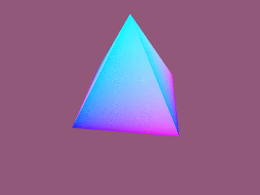
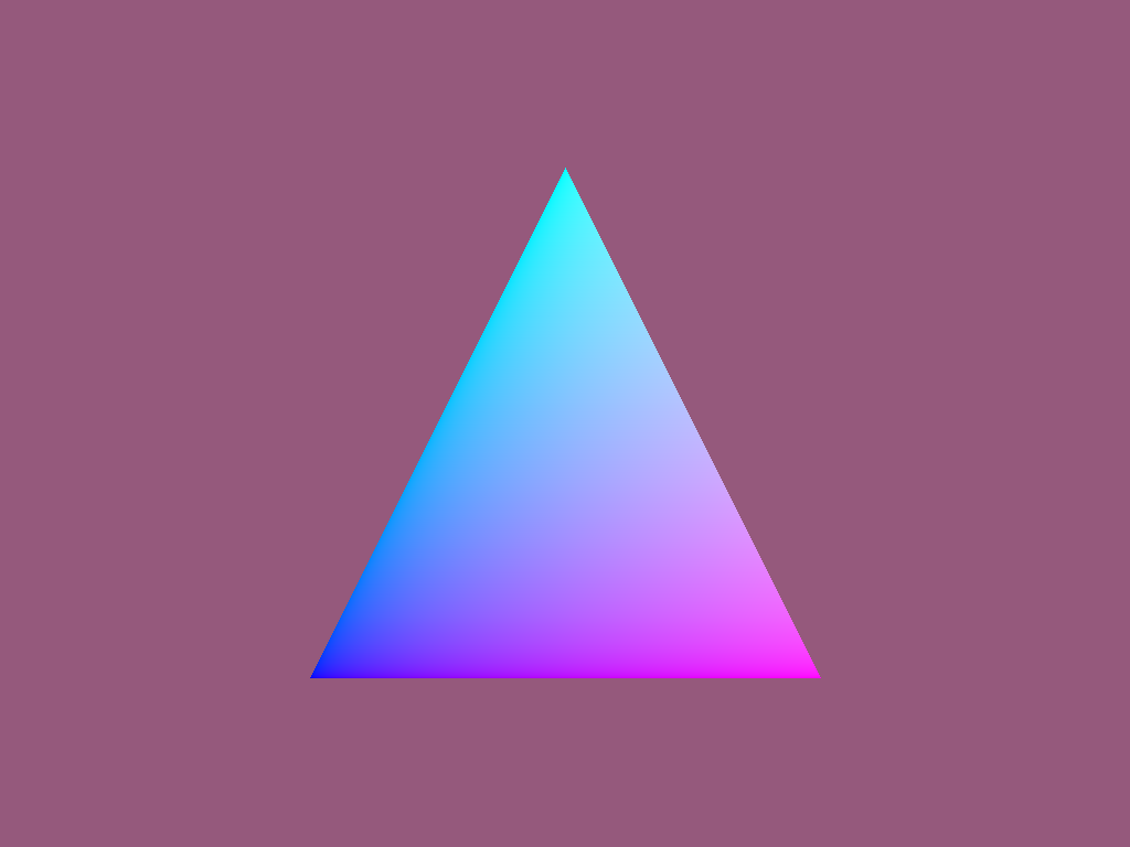
Figure 4 shows the final rendered result.
Summary
PyOptiX enables you to set up a ray-tracing rendering pipeline with Python. Numba converts Python functions into device code compatible with the rendering pipeline. NVIDIA combined these two libraries into the Numba extension for PyOptiX, enabling you to write accelerated ray-tracing applications in a full Python environment.
Combined with the rich and active environment that Python already enjoys, you now unlock the real power to build ray-tracing applications, hardware-accelerated. Download the demo to experiment with the Numba extension for PyOptiX yourself!
What’s next?
The PyOptiX Numba extension is at the development stage, and NVIDIA is working to add more examples and make typings for NVIDIA OptiX primitives more flexible and Pythonic.
What will you create? A game? A film? Or the VR application that you dreamt about? Share it in the comments!