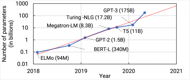
Scaling Language Model Training to a Trillion Parameters Using Megatron

Natural Language Processing (NLP) has seen rapid progress in recent years as computation at scale has become more available and datasets have become larger. At the same time, recent work has shown large language models to be effective few-shot learners, with high accuracy on many NLP datasets without additional finetuning. As a result, state-of-the-art NLP models have grown at an exponential rate (Figure 1). Training such models, however, is challenging for two reasons:

It is no longer possible to fit model parameters in the main memory of even the largest GPU.
Even if the model can be fitted in a single GPU (for example, by swapping parameters between host and device memory), the high number of compute operations required can result in unrealistically long training times without parallelization. For example, training a GPT-3 model with 175 billion parameters would take 36 years on eight V100 GPUs, or seven months with 512 V100 GPUs.

Sizes of state-of-the-art NLP models have increased by more than three orders of magnitude from 2018 to 2021. — *Figure 1. Trend of state-of-the-art NLP model sizes with time.*

In our previous post on Megatron, we showed how tensor (intralayer) model parallelism can be used to overcome these limitations. Although this approach works well for models of sizes up to 20 billion parameters on DGX A100 servers (with eight A100 GPUs), it breaks down for larger models. Larger models need to be split across multiple DGX A100 servers, which leads to two problems:

The all-reduce communication required for tensor model parallelism needs to go through inter-server links, which are slower than the high-bandwidth NVLink links available within a DGX A100 server
A high degree of model parallelism can lead to small GEMMs, potentially decreasing GPU utilization.

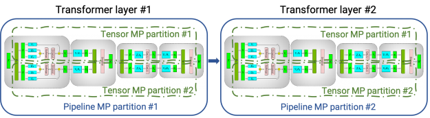
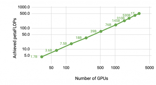
A model with two transformer layers can be split over 4 GPUs using both tensor and pipeline model parallelism. — Figure 2. Model parallelism for model with two transformer layers. Transformer layers are partitioned over pipeline stages (pipeline parallelism); each transformer layer is also split over 2 GPUs using tensor model parallelism.

To overcome these limitations, we combined tensor model parallelism with pipeline (interlayer) (model) parallelism. Pipeline parallelism was initially used in PipeDream and GPipe, and is now also available in systems such as DeepSpeed. We used tensor model parallelism inside a DGX A100 server and pipeline parallelism across DGX A100 servers. Figure 2 shows this combination of tensor and pipeline model parallelism. By combining these two forms of model parallelism with data parallelism, we can scale up to models with a trillion parameters on the NVIDIA Selene supercomputer (Figure 3). Models in this post are not trained to convergence. We only performed a few hundred iterations to measure time per iteration.

We saw an aggregate throughput improvement of 114x when moving from a ~1-billion-parameter model on 32 GPUs to a ~1-trillion-parameter model on 3072 A100 GPUs. Using 8-way tensor parallelism and 8-way pipeline parallelism on 1024 A100 GPUs, the GPT-3 model with 175 billion parameters can be trained in just over a month. On a GPT model with a trillion parameters, we achieved an end-to-end per GPU throughput of 163 teraFLOPs (including communication), which is 52% of peak device throughput (312 teraFLOPs), and an aggregate throughput of 502 petaFLOPs on 3072 A100 GPUs.

Aggregate achieved throughput increases by more than 100x when moving from a 1.7-billion-parameter model on 32 A100 GPUs, to a 1-trillion-parameter model on 3072 A100 GPUs. — *Figure 3. Achieved total petaFLOPs as a function of number of GPUs and model size. For model configuration details, see the “End-to-End Performance” section in this post.*

Our implementation is open source on the NVIDIA/Megatron-LM GitHub repository, and we encourage you to check it out! In this post, we describe the techniques that allowed us to achieve these results. For more information, see our paper, Efficient Large-Scale Language Model Training on GPU Clusters.

Pipeline parallelism

With pipeline parallelism, the layers of a model are partitioned across multiple devices. When used on repetitive transformer-based models, each device can be assigned an equal number of transformer layers. A batch is split into smaller microbatches; execution is then pipelined across microbatches. To retain vanilla optimizer semantics, we introduce periodic pipeline flushes so that optimizer steps are synchronized across devices. At the start and end of every batch, devices are idle. We call this idle time the pipeline bubble and want to make it as small as possible.

There are several possible ways of scheduling forward and backward microbatches across devices, and each approach offers different tradeoffs between pipeline bubble size, amount of communication, and memory footprint. We discuss two such approaches in this post.

Default schedule

GPipe proposes a schedule where the forward passes for all microbatches in a batch are first executed, followed by backward passes for all microbatches. Figure 4 shows a picture of this schedule. This approach has a high memory footprint as it requires stashed intermediate activations (or just input activations for each pipeline stage when using activation recomputation) for all microbatches in a batch. For the large batch sizes that are typically required to amortize away the cost of the pipeline bubble, this schedule is impractical due to its high memory footprint.

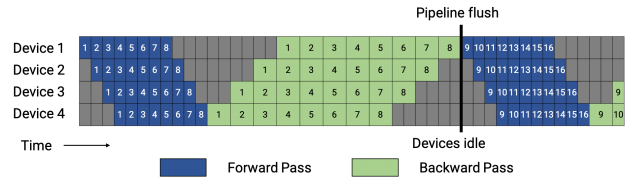
GPipe first schedules forward passes for all microbatches in a batch, followed by backward passes for all microbatches in a batch between pipeline flushes. — *Figure 4. Pipeline schedule with forward passes (blue) for all microbatches (represented by numbers) followed by backward passes (green). The gray area represents the pipeline bubble time.*

In Figure 4, for simplicity, we assumed that the backward pass takes twice as long as forward pass (wgrad, dgrad). The efficiency of the pipeline schedule is independent of this ratio. Each batch in this example consists of eight microbatches, and the number in each box is a unique identifier given to a microbatch. The optimizer is stepped, and weight parameters updated at the pipeline flush.

Instead, we used the PipeDream-Flush schedule. In this schedule, workers first enter a warm-up phase (Figure 5). This schedule limits the number of in-flight microbatches (the number of microbatches for which the backward pass is outstanding and activations need to be maintained) to the depth of the pipeline, instead of the number of microbatches in a batch. After the warm-up phase, each worker then enters steady state, where workers perform one forward pass followed by one backward pass (1F1B for short). Finally, at the end of a batch, workers complete backward passes for all remaining in-flight microbatches.

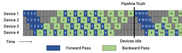
With the 1F1B schedule, workers can alternate between performing forward and backward passes for different microbatches in steady state. — *Figure 5. Pipeline schedule with 1F1B schedule (initial warm-up followed by a forward plus a backward pass for some microbatch in steady state).*

You can quantify the pipeline bubble size ( $t_{pb}$ ). Denote the number of microbatches in a batch as $m$ , the number of pipeline stages (equal to the number of devices used for pipeline model parallelism) as $p$ , the ideal time per iteration as $t_{id}$ , and the time to execute a single microbatch’s forward and backward pass as $t_f$ and $t_b$ . For the schedules in Figures 4 and 5, the pipeline bubble consists of $p-1$ forward passes at the start of a batch, and $p-1$ backward passes at the end. The total amount of time spent in the pipeline bubble is then:

$t_{pb} = (p-1) \cdot (t_f + t_b)$

The ideal processing time for a batch is:

$t_{id} = m \cdot (t_f + t_b)$

Therefore, the fraction of total time spent in the pipeline bubble can be computed as:

$\text{bubble time fraction} = \dfrac{t_{pb}}{t_{id}} = \dfrac{p-1}{m}$

For the bubble time fraction to be small, $m$ must be much larger than $p$ . The number of outstanding forward passes in this schedule is at most the number of pipeline stages. As a result, this schedule requires activations to be stashed for $p$ or fewer microbatches (compared to $m$ microbatches for the schedule in Figure 4). When $m \gg p$ , the schedule in Figure 5 is consequently much more memory-efficient than the one in Figure 4. Both schedules have the same pipeline bubble size.

Interleaved schedule

To reduce the size of the pipeline bubble, each device can perform computation for multiple subsets of layers (called a model chunk), instead of a single contiguous set of layers. For example, four layers of computation on each device can be split into two model chunks, each with two layers, instead of each device having a contiguous set of layers (device 1 has layers 1-4, device 2 has layers 5-8, and so on). With this scheme, each device in the pipeline is assigned multiple stages.

As before, you can use an all-forward, all-backward version of this schedule, but this has a high memory footprint. Instead, we developed a more memory-efficient, 1F1B version of this interleaved schedule. This new schedule is shown in Figure 6 and requires the number of microbatches in a batch to be an integer multiple of the degree of pipeline parallelism (number of devices in the pipeline). For example, with four devices, the number of microbatches in a batch must be a multiple of 4.

As shown in Figure 6, the pipeline flush for the same batch size happens sooner in the new schedule. If each device has $v$ stages (or model chunks), then the forward and backward time for a microbatch for each stage will now be $t_f / v$ and $t_b / v$ , respectively. Thus, the pipeline bubble time reduces to:

$\text{bubble time} = \dfrac{(p-1)\cdot(t_f + t_b)}{v}$

Each device can be assigned multiple stages, reducing the total amount of time the last device needs to wait for the first forward pass in a batch to start, and the last backward pass in a batch to complete. — Figure 6: Interleaved 1F1B schedule, where each device is assigned multiple stages (in this case, 2). Dark colors show the first stage and light colors show the second stage. Additional communication is required since the number of stages is doubled, but the size of the pipeline bubble is decreased (the pipeline flush happens sooner in the interleaved timeline assuming communication is free).

This reduced pipeline bubble size, however, does not come for free: this schedule requires extra communication. Quantitatively, the amount of communication increases by $v$ since the total number of stages also increases by $v$ . In the next section, we discuss how to use the eight InfiniBand networking cards in a DGX A100 node to reduce the impact of this extra communication.

Optimized internode communication using DGX A100 8 InfiniBand networking cards

In a pipelined setup, tensors must be sent and received in the forward and backward direction in parallel. Each DGX A100 is equipped with eight InfiniBand (IB) networking cards. Unfortunately, sends and receives are point-to-point, and only happen between a pair of GPUs on two servers. This makes it hard to leverage all eight cards in a single communication call.

However, you can make use of the fact that you want to use both tensor model parallelism and pipeline model parallelism to reduce the overhead of cross-node communication. The output of each transformer layer is replicated across the tensor-parallel ranks (Figure 4 from the Megatron paper). As a result, ranks in two consecutive pipeline stages that are performing tensor model parallelism send and receive the exact same set of tensors.

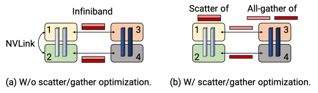
Without the scatter/gather optimization, the same tensor is sent redundantly over internode IB links. Instead, at the sender, you can scatter the tensor into smaller chunks, reducing the sizes of tensors sent over IB links. The final tensor can then be rematerialized at the receiver using all-gather over NVLink. — *Figure 7. Scatter/gather communication optimization to reduce the total number of bytes sent between GPUs on different multi-GPU servers.*

For large enough models, we used a tensor-model-parallel size of 8. This means that the same set of tensors are sent eight times between corresponding GPUs on adjacent multi-GPU servers. To reduce this redundancy, we instead split the tensor on the send side into equal-sized chunks and then only sent the chunk to the corresponding rank on the next node, using the rank’s dedicated IB card. With eight tensor-model-parallel ranks, each chunk is 8x smaller.

On the receiver side, to re-materialize the full tensor, we performed an all-gather over NVLink, which is much faster than the IB interconnect (Figure 7). We call this the scatter/gather communication optimization. This optimization helps better leverage the multiple IB cards on the DGX A100 servers and makes more communication-intensive schedules feasible, such as the interleaved one. The chunking optimization used here is like the activation partitioning technique to reduce memory footprint and pipeline-parallel communication from ZeRO and DeepSpeed.

Performance microbenchmarks for pipeline parallelism

In this section, we evaluated the computational performance of these pipeline-parallel schemes. This section does not use data parallelism, but we show results with both data and model parallelism later in this post.

Weak-scaling of pipeline parallelism

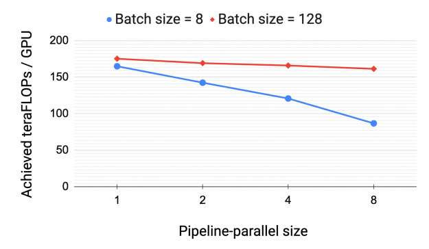
We first evaluated the weak-scaling performance of the default non-interleaved pipeline-parallel schedule using a GPT model with 128 attention heads, a hidden size of 20480, and a microbatch size of 1. As we increased the number of pipeline stages, we also increased the size of the model by proportionally increasing the number of layers in the model. For example, with a pipeline-parallel size of 1, we used a model with three transformer layers and ~15 billion parameters. With a pipeline-parallel size of 8, we used a model with 24 transformer layers and ~121 billion parameters. We used a tensor-parallel size of 8 for all configurations and varied the total number of A100 GPUs used from 8 to 64.

Figure 8 shows throughput per GPU for two different batch sizes. The peak device throughput of an A100 GPU is 312 teraFLOPs. As expected, the higher batch size scales better because the pipeline bubble is amortized over more microbatches (equal to batch size).

Throughput per GPU when using pipeline parallelism decreases with the increase in pipeline-parallel size. Smaller batch sizes see larger decreases. — *Figure 8. Throughput per GPU of pipeline parallelism using two different batch sizes in a weak-scaling experiment setup. Model size increases with the pipeline-parallel size.*

The number of floating point operations (numerator of throughput) is computed analytically based on the model architecture, taking activation recomputation into account.

Tensor vs. pipeline parallelism

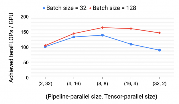
We also evaluated the impact of parallelization configuration on performance for a given model and batch size. The empirical results in Figure 9 show the importance of using both tensor and pipeline model parallelism in conjunction to train a 161-billion-parameter GPT model (32 transformer layers, 128 attention heads, hidden size of 20480) with low communication overhead and high compute resource utilization. Tensor model parallelism is best within a node (DGX A100 server) due to its expensive all-reduce communication.

Pipeline model parallelism, on the other hand, uses much cheaper point-to-point communication that can be performed across nodes without bottlenecking the entire computation. However, pipeline parallelism can spend significant time in the pipeline bubble. The total number of pipeline stages should thus be limited so that the number of microbatches in the pipeline is a reasonable multiple of the number of pipeline stages. Consequently, we saw peak performance when the tensor-parallel size was equal to the number of GPUs in a single node (8 on Selene with DGX A100 nodes).

When using both pipeline and tensor model parallelism, throughput per GPU depends on both the size of the pipeline bubble, and the amount of expensive cross-node communication. Across batch sizes, you see highest throughput for pipeline-parallel size = 8, tensor-parallel size = 8. — Figure 9. Throughput per GPU of various parallel configurations that combine pipeline and tensor model parallelism using a GPT model with 162.2 billion parameters, two different batch sizes, and 64 A100 GPUs.

Scatter-gather optimization for communication

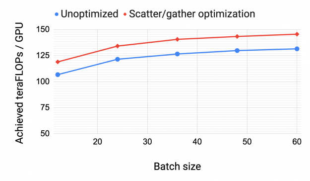
Figure 10 shows per-GPU throughput with and without (unoptimized) the scatter/gather communication optimization for a GPT model with 175 billion parameters (96 attention heads, hidden size of 12288, and 96 transformer layers). End-to-end throughput improves by up to 11% for communication-intensive schedules (large batch size with interleaving). This highlights the importance of the DGX A100 eight IB cards in achieving high training throughput for large models.

The scatter/gather optimization improves throughput by up to 11% across a range of batch sizes with the interleaved schedule. — *Figure 10. Throughput per GPU with and without the scatter/gather optimization for a GPT model with 175 billion parameters using 96 A100 GPUs and the interleaved schedule.*

Interleaved vs. non-interleaved schedule

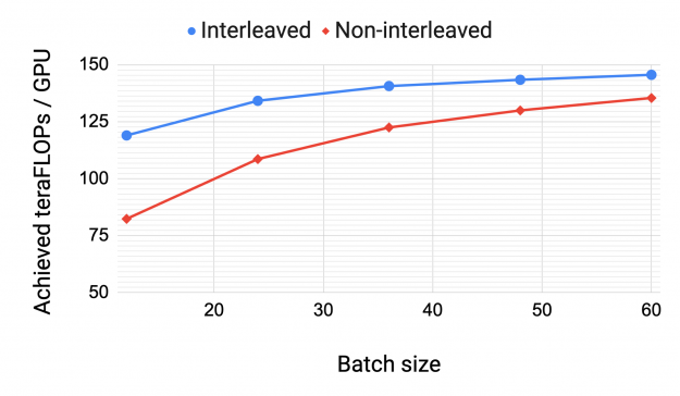
Figure 11 shows the per-GPU throughput for interleaved and non-interleaved schedules on the same GPT model with 175 billion parameters. The interleaved schedule with the scatter/gather communication optimization has higher computational performance than the non-interleaved (default) schedule. This gap closes as the batch size increases, due to two reasons:

As the batch size increases, the bubble size in the default schedule decreases.
The amount of point-to-point communication within the pipeline is proportional to the batch size. Consequently, the non-interleaved schedule catches up as the amount of communication increases.

Without the scatter/gather optimization, the default schedule performs better than the interleaved schedule at larger batch sizes (not shown).

For a GPT model with 175 billion parameters, the interleaved schedule has higher per-GPU throughput than the non-interleaved schedule across batch sizes. The gap between the two schedules decreases as the batch size increases. — *Figure 11. Throughput per GPU of interleaved and non-interleaved schedules for a GPT model with 175 billion parameters using 96 A100 GPUs.*

End-to-end scaling using model and data parallelism

Consider the weak-scaling performance of Megatron on GPT models ranging from a billion to a trillion parameters. We used tensor, pipeline, data parallelism, and the interleaved pipeline schedule with the scatter/gather optimization enabled. All models used a vocabulary size of 51,200 (multiple of 1024) and a sequence length of 2048. We varied the hidden size, number of attention heads, and number of layers to arrive at a specific model size. As the model size increased, we also increased the batch size and the number of GPUs.

Table 1 shows the model configurations along with the achieved FLOPs per second (both per GPU and aggregate over all GPUs). We saw almost-perfect linear scaling to 3072 A100 GPUs (384 DGX A100 nodes), as shown in Figure 1. Throughput is measured for end-to-end training: all operations including data loading, optimization, and logging. The largest case achieves 52% of the theoretical peak FLOPs.

Model size	Hidden size	Number of layers	Model-parallel size	Number of GPUs	Batch size	Achieved teraFlOPs per GPU
1.7B	2304	24	1	32	512	137
3.6B	3072	30	2	64	512	138
7.5B	4096	36	4	128	512	142
18B	6144	40	8	256	1024	135
39B	8192	48	16	512	1536	138
76B	10240	60	32	1024	1792	140
145B	12288	80	64	1536	2304	148
310B	16384	96	128	1920	2160	155
530B	20480	105	280	2520	2520	163
1T	25600	128	512	3072	3072	163

Table 1. Weak-scaling throughput for GPT-3 models ranging from 1 billion to 1 trillion parameters.

Finally, based on the measured throughputs from Table 1, you can estimate the training time. The time required to train a GPT-based language model with $P$ parameters using $T$ tokens on $N$ GPUs with per-GPU throughput of $X$ can be estimated as follows:

$\text{Training time (seconds)} \approx 8 \cdot \dfrac{TP}{NX}.$

For the 1 trillion parameter model, assume that you need about 450 billion tokens to train the model. Using 3072 A100 GPUs with 163 teraFLOPs / GPU, you require:

$\text{1T model training time} \approx 8 \cdot \dfrac{450 \times 10^9 \times 1008 \times 10^9}{3072 \times 163 \times 10^{12}} \approx 84 \text{ days},$

This is less than three months. The GPT-3 model with 175 billion parameters requires just over a month to train using 1024 A100 GPUs. These results indicate that it is feasible to train such large models in a reasonable amount of time with this system. For more information, see Efficient Large-Scale Language Model Training on GPU Clusters.

Summary

In this post, we outlined various techniques that facilitate the training of NLP models with up to a trillion parameters, using a smart combination of different parallelization strategies:

Intranode tensor model parallelism
Internode pipeline model parallelism
Data parallelism

Going forward, we want to further optimize our pipelining schedules. For example, we expect a throughput improvement if we can compute data gradients before weight gradients, as tensors can be sent upstream earlier, leading to a cheaper pipeline flush. We also want to explore the tradeoffs associated with hyperparameters such as microbatch size, global batch size, and the degree of activation recomputation on throughput. Finally, we want to train models to convergence, and better understand the implications of using schedules without pipeline flushes, such as PipeDream-2BW, which has relaxed weight update semantics.