[This post was co-written by Everett Phillips and Massimiliano Fatica.]
The High Performance Conjugate Gradient Benchmark (HPCG) is a new benchmark intended to complement the High-Performance Linpack (HPL) benchmark currently used to rank supercomputers in the TOP500 list. This new benchmark solves a large sparse linear system using a multigrid preconditioned conjugate gradient (PCG) algorithm. The PCG algorithm better represents the computational and communication patterns prevalent in modern application workloads which rely more heavily on memory system and network performance than HPL.
GPU-accelerated supercomputers have proven to be very effective for accelerating compute-intensive applications like HPL, especially in terms of power efficiency. Obtaining good acceleration on the GPU for the HPCG benchmark is more challenging due to the limited parallelism and memory access patterns of the computational kernels involved. In this post we present the steps taken to obtain high performance of the HPCG benchmark on GPU-accelerated clusters, and demonstrate that our GPU-accelerated HPCG results are the fastest per-processor results reported to date.
The PCG Algorithm
The PCG algorithm solves a sparse linear system \(\mathbf{A}\mathbf{x} = \mathbf{b}\) given an initial guess \(\mathbf{x}_0\). The particular sparse linear system used in HPCG is a simple elliptic partial differential equation discretized with a 27-point stencil on a regular 3D grid. Rows in the sparse matrix \(\mathbf{A}\) represent points in the grid. Each processor is responsible for a subset of rows corresponding to a local domain of size \(N_{x} \times N_{y} \times N_{z}\), chosen by the user in the setup file. The number of processors is automatically detected at runtime, and decomposed into \(P_{x} \times P_{y} \times P_{z}\), where \(P=P_{x}P_{y}P_{z}\) is the total number of processors. This creates a global domain \(G_{x} \times G_{y} \times G_{z}\), where \(G_{x} = P_{x}N_{x}, G_{y} = P_{y}N_{y},\) and \(G_{z} = P_{z}N_{z}\). Although the matrix has a simple structure, it is only intended to facilitate the problem setup and validation of the solution. Implementations may not use assumptions about the matrix structure to optimize the solver; they must treat the matrix as a general sparse matrix.
Following is pseudocode for the PCG algorithm.
\(k := 0\)
Compute the residual \(\mathbf{r}_0 := \mathbf{b} - \mathbf{A}x_0\)
while (\(||\mathbf{r}_{k}|| < \epsilon\))
    \(\mathbf{z}_{k} := \mathbf{M}^{-1}\mathbf{r}_{k}\)
    \(k = k+1\)

    if (k==1)
        \(\mathbf{p}_1 := \mathbf{z}_0\)
    else
        \(\beta_{k} := (\mathbf{r}_{k-1}^\top \mathbf{z}_{k-1}) / (\mathbf{r}_{k-2}^\top \mathbf{z}_{k-2})\)
        \(\mathbf{p}_{k} := \mathbf{z}_{k-1} + \beta_{k}p_{k-1}\)
    end if

    \(\alpha_{k} := (\mathbf{r}_{k-1}^\top\mathbf{z}_{k-1}) / (\mathbf{p}_{k}^\top\mathbf{A}\mathbf{p}_{k})\)
    \(\mathbf{x}_{k} := \mathbf{x}_{k-1} + \alpha_{k}\mathbf{p}_{k}\)
    \(\mathbf{r}_{k} := \mathbf{r}_{k-1} - \alpha_{k}\mathbf{A}\mathbf{p}_{k}\)
end while

\(\mathbf{x} := \mathbf{x}_{k}\)
We can identify three basic operations:
- Application of the preconditioner \(\mathbf{w} := \mathbf{M}^{-1}\mathbf{y}\), where \(\mathbf{M}^{-1}\) is an approximation to \(\mathbf{A}^{-1}\). In HPCG, the preconditioner is an iterative multigrid solver using a symmetric Gauss-Seidel smoother (SYMGS). Application of SYMGS at each grid level involves neighborhood communication, followed by local computation of a forward sweep (update elements in row order) and backward sweep (update elements in reverse row order) of Gauss-Seidel. Each of the sweeps acts like a sparse triangular solver, and applies the matrix to the current approximation of the solution, one row at a time. This ordering constraint makes the SYMGS routine difficult to parallelize, and is the main challenge of the HPCG benchmark.
- Sparse matrix-vector (SPMV) products \(\mathbf{Ay}\). This operation requires neighborhood communication to collect the remote values of \(\mathbf{y}\) owned by neighbor processors, followed by multiplication of the local matrix rows with the input vector. The pattern of computation is similar to a sweep of SYMGS, however the output vector is distinct from the input vector, so all matrix rows can be trivially processed in parallel.
- Vector inner products (DOT) \(\mathbf{a} := \mathbf{y}^\top\mathbf{z}\). Each MPI process computes its local inner product and then calls a collective reduction to get the final value.
All of the routines are vector-vector (BLAS1) or sparse matrix-vector (BLAS2) operations, with low compute intensity (ratio of floating point operations to memory access).
The HPCG Benchmark
After the initial setup and validation, the benchmark calls a user-defined optimization routine, which allows for analysis of the matrix, reordering of the matrix rows, and transformation of data structures, in order to expose parallelism and improve performance of the SYMGS smoother. This generally requires reordering matrix rows using graph coloring for performance on highly parallel processors such as GPUs. However, this introduces a slowdown in the rate of convergence, which in turn increases the number of iterations required to reach the solution. The time for these additional iterations, as well as the time for the optimization routine, is counted against the final performance result.
Next, the benchmark calls the reference PCG solver for 50 iterations and stores the final residual. The optimized PCG is then executed for one cycle to find out how many iterations are needed to match the reference residual. Once the number of iterations is known, the code computes the number of PCG sets required to fill the entire execution time. The benchmark can complete in a matter of minutes, but official results submitted to Top500 require a minimum of one hour duration.
CUDA Implementation of HPCG
Our GPU porting strategy focused on parallelizing the Symmetric Gauss-Seidel smoother (SYMGS), which accounts for approximately two thirds of the benchmark flops. This function is difficult to parallelize due to the data dependencies imposed by the ordering of the matrix rows. Although it is possible to expose a moderate amount of parallelism using analysis of the matrix structure to build a dependency graph, for GPUs it is more effective to reorder the rows using graph coloring. Our efficient graph coloring implementation (based on earlier work by Jonathan Cohen) accounts for a very small fraction of overall run time.
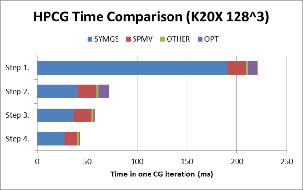
Our implementation begins with a baseline using CUDA libraries, and progresses into our final version in the following steps:
- cuSPARSE
- cuSPARSE + reordering
- Custom Kernels + reordering
- Custom Kernels + reordering + ELLPACK matrix format
We achieved best results with matrix reordering, and by storing the matrix in ELLPACK format, which enables coalesced memory access to the matrix elements. We also overlap communications with computations to improve scaling on large systems.
Figure 1 shows performance improvements over the four optimization phases.
HPCG on a Single GPU
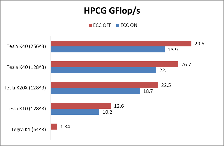
HPCG reports results in GFlop/s, but the benchmark performance reflects memory system performance. By running the code on different classes of GPUs, from the smallest CUDA-capable GK20A found in the Tegra K1 to the Tesla K40, we were able to study the correlation between memory system and HPCG performance. The benchmark performs all computations in double precision. The following table summarizes the technical specification of the GPUs used in our study, and Figures 2 and 3 show HPCG and STREAM performance of the GPUs, respectively.
| Processor | #SMs | # Cores fp32/fp64 |
Core Clock (MHz) |
fp64 Peak (GFlop/s) |
Memory Clock (MHz) |
Memory bus width |
Memory Bandwidth (GB/s) |
|---|---|---|---|---|---|---|---|
| Tegra K1 | 1 | 192/8 | 852 | 13.6 | 924 | 64-bit | 14.7 |
| Tesla K10 | 8 | 1536/64 | 745 | 95 | 2500 | 256-bit | 160 |
| Tesla K20x | 14 | 2688/896 | 732 | 1310 | 2600 | 384-bit | 250 |
| Tesla K40 | 15 | 2880/960 | 875 | 1680 | 3000 | 384-bit | 288 |

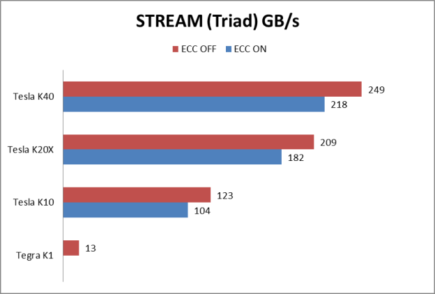
If we look at the table of results, we see a strong correlation between the HPCG result and the sustained memory bandwidth measured by the STREAM benchmark.
| NVIDIA GPU | Size | HPCG GFlop/s | Stream GB/s | HPCG/Stream |
|---|---|---|---|---|
| Tegra K1 | 643 | 1.34 | 13 | 0.103 |
| Tesla K10 | 1283 | 12.6 | 123 | 0.102 |
| Tesla K20x | 1283 | 22.5 | 209 | 0.107 |
| Tesla K40 | 1283 | 26.7 | 249 | 0.107 |
Figure 4 plots the HPCG performance versus the STREAM bandwidth. We can see that there is an excellent fit among all the different processors, including the CPU implementation.
![Figure 4: Correlation between HPCG performance and STREAM bandwidth. CPU Results from [TODO: Add citation/link]](/blog/wp-content/uploads/2014/07/HPCG_Figure4_HPCGvsSTREAM-624x364.png)
HPCG on Multiple Nodes
When running on multiple nodes, the network plays a key role in overall HPCG performance. This is what makes HPCG an interesting benchmark (otherwise it would just be a STREAM benchmark in disguise).
There are two distinct phases of communication, the first involving the exchange of boundary data with neighboring processes in the SYMGS and SPMV routines, and the second related to the global reductions required by the DOT (dot product) routine. For the first phase, it is possible to hide the communication with computation, but the global reduction in the second phase is more difficult to overlap, and scales as the logarithm of the number of nodes. This is exactly what we can see in Figure 5, which plots communication overhead in the runs performed on the Titan supercomputer at Oak Ridge National Labs.
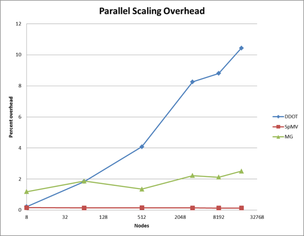
Our current implementation completely overlaps communication with computation for the sparse matrix vector product (red line). We have not yet attempted overlap in the multigrid phase (green line), but we can see that on Titan’s 3D torus network this communication has nearly constant overhead. The MPI_Allreduce() calls needed to compute dot products (blue line) become the largest overhead at full scale, accounting for more than 10% of the run time.
Analysis of the First HPCG List
The first HPCG list was published at ISC14 and included 15 supercomputers. Instead of looking at the peak flops of these machines, we evaluate the efficiency based on the ratio of the HPCG result to the memory bandwidth of the processors. The following table shows the results of the top 4 systems that submitted optimized results.
| HPCG Rank | Machine Name | HPCG GFlop/s | #Procs | Processor Type | HPCG per Proc | Bandwidth per Proc | Efficiency (flops/byte) |
|---|---|---|---|---|---|---|---|
| 1 | Tianhe-2 | 580,109 | 46,080 | Xeon Phi-31S1P | 12.59 GF | 320 GB/s | 0.039 |
| 2 | K | 426,972 | 82,944 | Sparc64-viiifx | 5.15 GF | 64 GB/s | 0.080 |
| 3 | Titan | 322,321 | 18,648 | Tesla-K20X+ECC | 17.28 GF | 250 GB/s | 0.069 |
| 5 | Piz Daint | 98,979 | 5,208 | Tesla-K20X+ECC | 19.01 GF | 250 GB/s | 0.076 |
As we can see from the HPCG per processor column, the GPU-accelerated clusters are the fastest architecture for HPCG. The comparison between Piz-Daint and Titan shows the improvement of the new Aries dragonfly interconnect used in Piz-Daint over the Gemini 3D torus network used in Titan. The performance of GPUs is also affected by ECC, which is not accounted for in the efficiency computation. (One system reported results without ECC: the Tsubame-KFC system achieved over 23 GFLOP/s per processor on 160 Tesla K20X GPUs).
Conclusions
These results show that GPU-accelerated clusters perform very well in the new HPCG benchmark. Our results are the fastest per processor ever reported. GPUs, with their excellent floating point performance and high memory bandwidth, are very well-suited to tackle workloads dominated by floating point, like HPL, as well as those dominated by memory bandwidth, like HPCG.
If you’d like to learn more about our work on HPCG, be sure to attend Everett Phillips’ talk in the NVIDIA Booth #1727 at Supercomputing 2014 on Tuesday, November 18 at 10:30am. To learn more about HPCG, attend the SC14 HPCG Birds-of-a-feather.