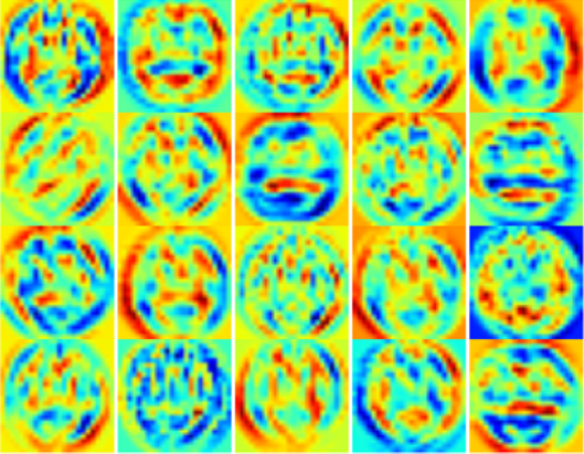
Pattern recognition and classification in medical image analysis has been of interest to scientists for many years. Machine learning techniques have enabled researchers to develop and utilize complicated models to classify or predict various abnormalities or diseases. Recently, the successful applications of state-of-the-art deep learning architectures have rapidly expanded in medical imaging. Cutting-edge deep learning tools such as NVIDIA DIGITS along with deep learning frameworks like Caffe, Torch or Theano help researchers concentrate on problem solving and model development rather than coding. We have had success using deep learning and NVIDIA DIGITS for Alzheimer’s Disease prediction.
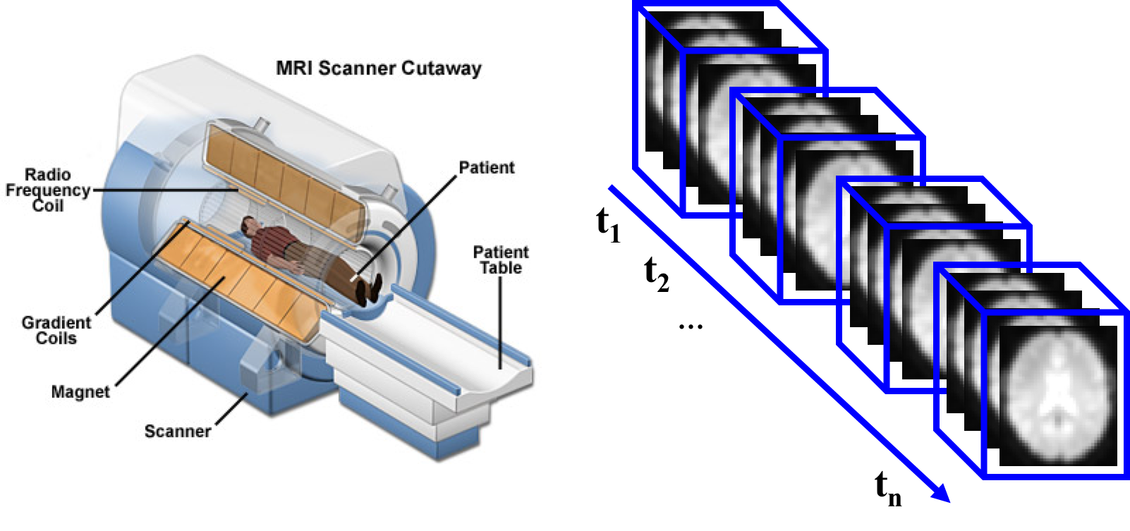
Research groups around the world have put a lot of effort into classifying and predicting Alzheimer’s disease from brain imaging data. Alzheimer’s is a type of dementia that causes problems with memory, thinking and behavior. Symptoms usually develop slowly and worsen over time, becoming severe enough to interfere with daily tasks. Statistics show that Alzheimer’s Disease (AD) is the 6th leading cause of death in the United States. The US spends almost $236 billion per year to care for around 5 million people suffering from this brain disorder.
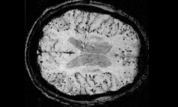
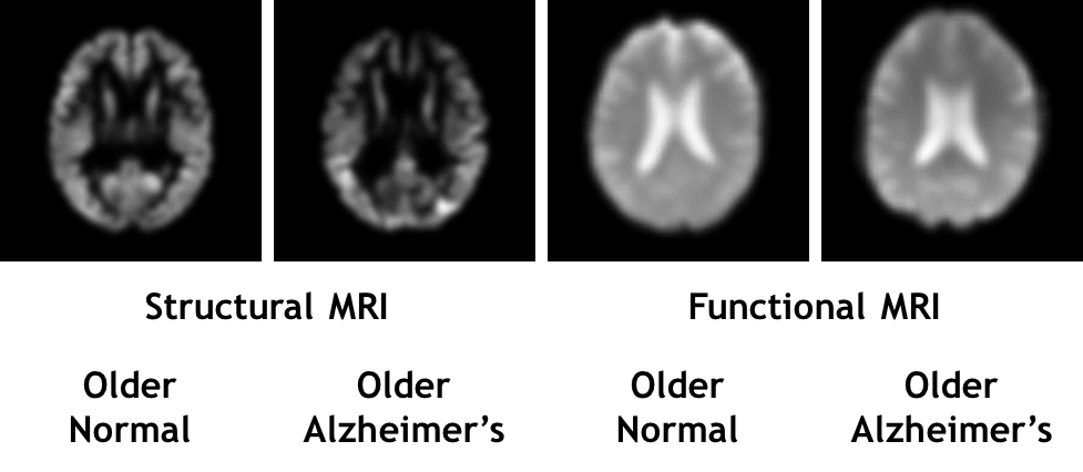
A variety of imaging modalities are used in both clinics and research to produce AD data, including structural Magnetic Resonance Imaging (MRI) as well as functional imaging modalities such as Positron Emission Tomography (PET) and functional MRI monitoring the functionality of the brain.
In this practical experience, we designed and implemented an end-to-end deep learning pipeline that includes several steps from preprocessing to prediction. We used NVIDIA DIGITS to train a Convolutional Neural Network model for Alzheimer’s Disease prediction from resting-state functional MRI (rs-fMRI) data.
Deep Learning Pipeline for Alzheimer’s Disease Prediction
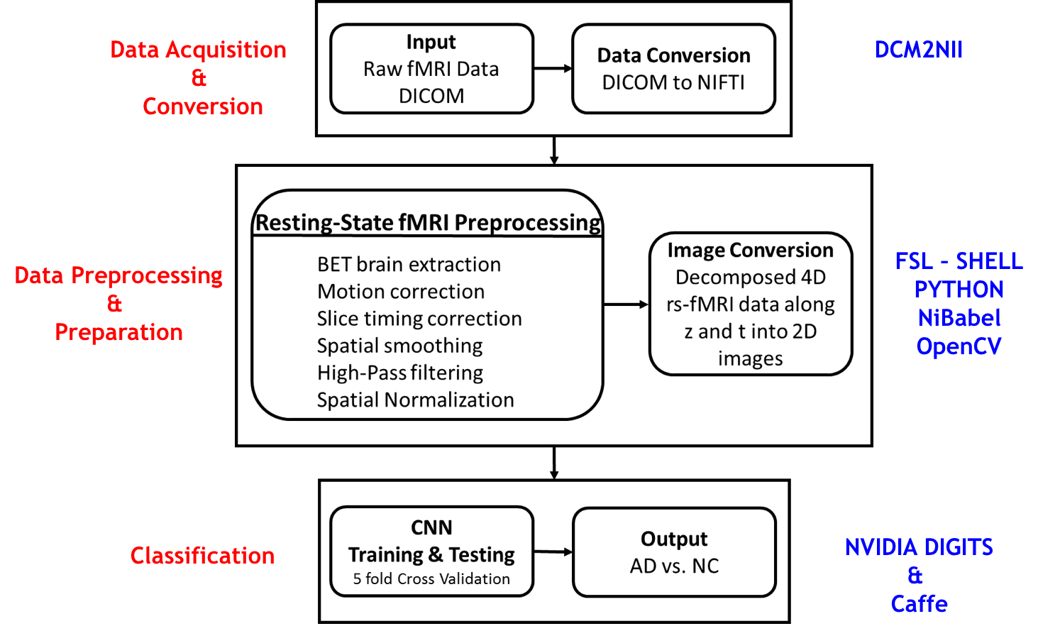
We designed the end-to-end pipeline shown in Figure 2 based on three major components. In the first layer, the rs-fMRI raw data (DICOM) is converted to a standard imaging format (NIfTI). The primary goal of NIfTI is to provide coordinated and targeted service, training, and research to speed the development and enhance the utility of informatics tools related to neuroimaging. The National Institute of Mental Health and the National Institute of Neurological Disorders and Stroke are joint sponsors of the NIfTI initiative. The next step preprocesses the rs-fMRI data (explained later) and converts it into a format readable by our deep learning platform: NVIDIA Caffe DIGITS. Finally, we trained, validated and tested a 2-layer convolutional neural network model from the standard LeNet-5 architecture using DIGITS. For further analysis, we passed the test dataset through the “classify many” option provided by DIGITS to obtain a class score per sample.
Data Acquisition and Preprocessing
In this work, we selected 28 Alzheimer’s Disease (AD) and 15 normal control (NC) subjects (24 female and 19 male) with a mean age of years from the ADNI1* dataset. The AD subjects’ Mini–Mental State Examination (MMSE) scores were reported to be over 20 by ADNI, and normal participants were healthy, with no reported history of medical or neurological conditions. Scanning was performed on a Trio 3 Tesla, which included structural and functional scans. First, anatomical scans were performed with a 3D MP-RAGE sequence (TR=2s, TE=2.63 ms, FOV=25.6 cm, 256 x 256 matrix, 160 slices of 1mm thickness). Next, functional scans were obtained with an EPI sequence (150 volumes, TR=2 s, TE=30 ms, flip angle=70, FOV=20 cm, 64 x 64 matrix, 30 axial slices of 5mm thickness, no gap). We pre-processed the fMRI data using the standard modules from the FMRIB Software Library v5.0. Preprocessing steps for the anatomical data involved the removal of non-brain tissue from T1 structural images using the Brain Extraction Tool. Preprocessing steps for the functional data included motion correction, skull stripping, and spatial smoothing (Gaussian kernel of 5-mm FWHM). We removed low-level noise using high-pass temporal filtering (= 90.0 sec), aligned functional images to individual high-resolution T1-weighted scans, and subsequently registered the scans to the Montreal Neurological Institute standard space (MNI152) using affine linear registration and resampled them at 2mm cubic voxels. The end results of the preprocessing step were 45x54x45x300 images, from which we removed the first 10 slices of each image, as they contained no functional information.
Data Conversion and Augmentation
We decomposed the preprocessed 4D fMRI data in NIfTI format across the z and t axes and then converted them to a stack of 2D images in lossless PNG format using the neuroimaging packages Nibabel and Python OpenCV. Next, we labeled the images for binary classification of Alzheimer’s vs. normal data. This conversion approach resulted in a fair number of samples. We removed the last 10 brain slices of each scan during the data conversion as brain imaging researchers showed that no functional information is often encoded in those brain slices (Table 1).
| Subjects | Slices | Volumes | Total |
| 43 | 35* | 300 | 451500 |
| Training | Testing | Validation |
| 60% | 20% | 20% |
| 270900 | 90300 | 90300 |
Experience with NVIDIA Caffe DIGITS
After completing the data augmentation, we used the samples to create Lightning Memory-Mapped Database Manager (lmdb) storage databases for high-throughput to be fed into a deep learning framework. DIGITS provides two options to users to convert the samples: either store the samples in different folders corresponding to the class labels or create custom text files listing the label for each sample. For simplicity, we used the first option provided by DIGITS by storing the samples into two folders AD and NC, for Alzheimer’s and Normal, respectively. DIGITS automatically created the training and testing lmdb datasets. Next, we selected the standard LeNet-5 model and initiated the training process. We used an Amazon AWS server image with NVIDIA GPUs, Caffe, and DIGITS already installed.
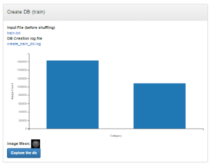
Figure 5 shows the process of creating a new imaging dataset. In our case, we created Grayscale 32×32 images in lossless PNG format and divided the data into training, validation and testing samples (60%, 20% and 20%, respectively). DIGITS shows the distribution of labels in the datasets using histograms, as Figure 4 shows. Once the datasets were created, we selected the LeNet model and then clicked “Customize” to visualize the topology of the network (Figure 6). The visualization option helped us better understand the implementation of the CNN model at a high-level. In general, the visualization helps neural network architecture designers aiming to develop and test a new model.
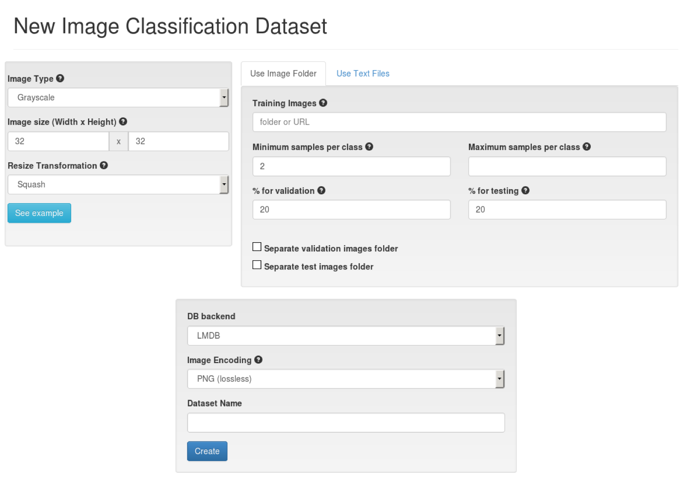
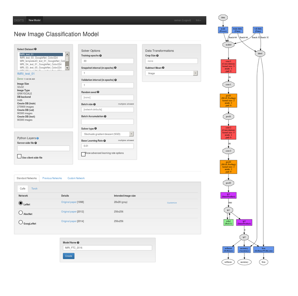
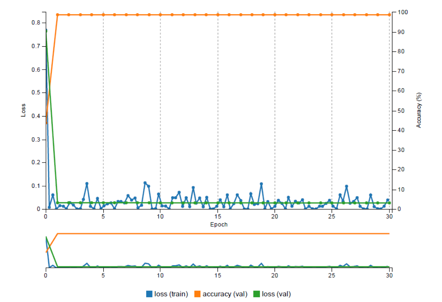
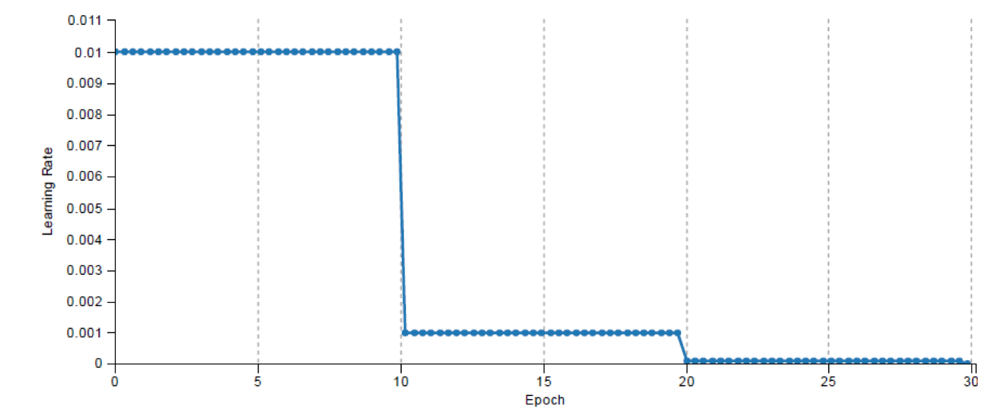
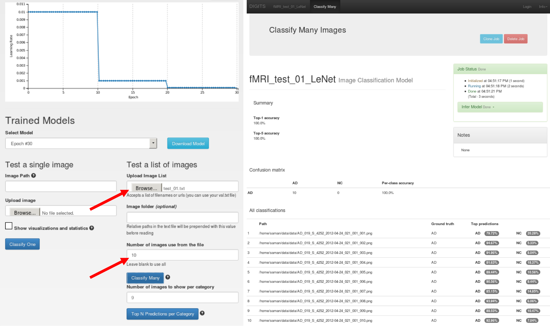
Figure 6: This figure illustrates the process of selecting a dataset and the LeNet neural network model (Left image). At right, the topology of the network is visualized.The beauty of using DIGITS as a training platform is the real-time monitoring of the network performance, which allowed us to carefully control the entire training process, visually analyze each epoch’s performance, and spot issues in the data and the training process. DIGITS also shows the Estimated Time of Completion (ETS), which helps predict when long training runs will complete. Figure 7 shows the DIGITS visualization of the network’s performance with a plot of the loss for the training and validation datasets and the accuracy achieved on the validation dataset over training epochs. Also, the graph in Figure 8 shows how the learning rate decreases over time. Users who have a deeper background in machine learning might be interested to see the effect of learning rate on the training process for further network analysis.
In this work, we were interested in obtaining the class scores per testing sample for further analysis. There are multiple methods for this, such as using the Caffe command-line API or the PyCaffe API. DIGITS provides a GUI-based option called “Classify Many” where you can upload a text file list of testing sample paths (you can use the test.txt file generated by DIGITS) and obtain the class scores for every sample in the list. You can also limit the number of samples from your text file that are tested. Figure 9 shows how to select the text file and the number of testing samples (in this case, we selected 10 samples). We saved the output as an HTML file and then converted it into an Excel format readable by any programming language such as Python and MATLAB which allowed us to perform more data mining and to generate ROC curves to investigate the performance of binary classification.
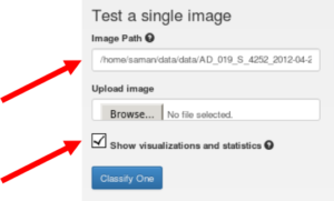
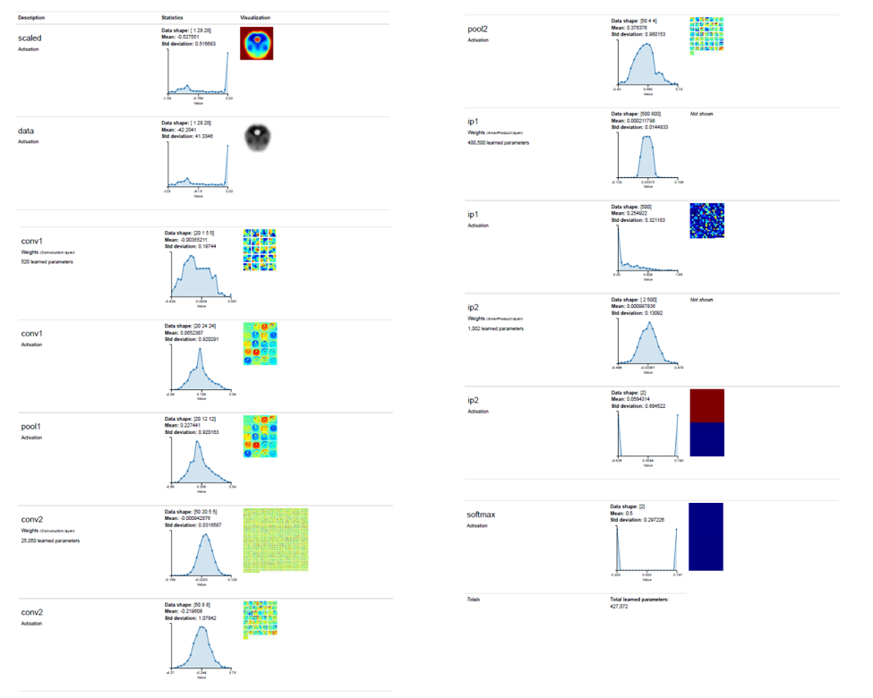
We also used the DIGITS “Classify One Image” option (Figure 10). Although the class scores can be obtained for all samples using the ‘Classify Many’ option, the visualization of certain preliminary or intermediary results for a given simple can be interesting and informative, as Figure 11 shows. This option creates a variety of results and visualizations that can be used in reports and publications, including the scaled input image, filters and feature weights, and pooling and softmax layer outputs. Additionally, you can use the DIGITS interface to download and save the Caffe model and then write a script to extract the filters and other network parameters.
ROC Curve
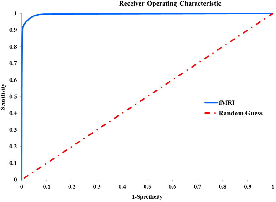
To validate the performance of the binary classification performed with the pipeline, we drew the Receiver Operating Characteristic (ROC) curve. Basically, ROC curves are plots of the true positive rate (or sensitivity) against the false positive rate (1-specificity) for the different possible thresholds of a classification test. We extracted the class scores for each sample using “Classify Many” as discussed previously and then calculated the true and false positive rates for 10 thresholds from zero to one with a step of 0.1 (0:1:0.01) as shown in the following equations. Figure 9 shows the ROC curve for validating the performance of the binary classification.
\(Sensitivity = True Positive Rate (TPR) = TP/p = TP/(TP+FN)\)
\(Specificity = True Negative Rate (TNR) = TN/N = TN/(FP+TN)\)
Results
We repeated the entire dataset generation and classification process five times for 5-fold cross validation, achieving an average accuracy rate of 96.85%. The end-to-end pipeline shows high reproducibility and consistency. We presented this deep learning experiment using DIGITS as “Deep Learning-based Pipeline to Recognize Alzheimer′s Disease using fMRI Data” in the Co-sponsored IEEE Future Technology Conference FTC2016 in San Francisco December 6 and 7th 2016, and won the best paper award. You can access our paper on IEEE Xplore.
Future Work
The upcoming project called “DeepAD” has begun by looking at both structural MRI and functional MRI data utilizing many more samples and various CNN models for classification. In addition to slice-level classification similar to the previous work, the project has performed subject-level classification followed by decision making. In addition, the project has investigated the effect of imbalanced data on CNN classification results. Figure 10 shows some preliminary results. We successfully showed how big data samples that were preprocessed carefully could achieve around 100% accuracy. Additionally, we developed decision making as a post-classifier on top of DIGITS results to purify the subject-level classification results.

Get Started with DIGITS Today!
DIGITS makes it easy to manage the design and training of deep neural networks. It also helps you create and manage training and validation data sets. You can download DIGITS today for free.
Learn about the powerful image segmentation features in DIGITS 5 in this in-depth post by Greg Heinrich. Learn about object detection with DIGITS in this post on DetectNet and this one on SpaceNet.
Acknowledgment
I would to thank Drs. Danielle D. DeSouza, John Anderson and Ghassem Tofighi and also Ms. Kristin Uchiyama for extending their help and support to make these projects and this tutorial happen.
*Data used in preparation of this article were obtained from the Alzheimer’s Disease Neuroimaging Initiative (ADNI) database (adni.loni.usc.edu). As such, the investigators within the ADNI contributed to the design and implementation of ADNI and/or provided data but did not participate in analysis or writing of this report. Here is a complete listing of ADNI investigators.
